Graphing Linear Relationships
Introduction
A table is a set of answers that has not yet shown its shape. When you place each input-output pair on a coordinate plane, a numerical pattern becomes something you can inspect, extend, and test.
You are beginning the fourth of five lessons in Linear Graphs, Slope, and Intercepts. In the first three lessons, you recognized linear relationships, described their constant change with slope, and interpreted intercepts; now you will use those ideas to construct a graph from the data itself.
By the end of this lesson, you will be able to:
- Convert each table row into an ordered pair.
- Plot points using the correct horizontal and vertical coordinates.
- Construct a visible line through two distinct points.
- Check that a line represents every pair in a table.
Begin by connecting three views of the same relationship: a table, a collection of points, and a straight graph.
Connect Tables, Points, and Graphs
Each row of a value table records one input-output result. Writing that row as an ordered pair places the result at a specific location on the coordinate plane.
| Representation | What it shows |
|---|---|
| Value table | Separate input-output results |
| Ordered pair | One result as a point |
| Linear graph | All the points and the straight path they share |
For a linear relationship, the output changes at one constant rate as the input changes. If is the slope, then the changes are connected by
Here, means a change in the input and means the corresponding change in the output. Even when table rows use different input intervals, the same rate keeps the points on one straight line.
Translate Table Rows into Ordered Pairs
With that connection in mind, read each table row from left to right. The first value is the horizontal coordinate, and the second value is the vertical coordinate.
| Input | Output | Ordered pair |
|---|---|---|
The values in a row belong together. For example, the input is paired with the output , so the point is , not . In a matching activity, compare both coordinates and preserve this input-output order.
Plot Points on the Coordinate Plane
After creating the ordered pairs, place each point using the same coordinate-reading routine:
- Start at the origin, .
- Move horizontally to the -coordinate: right for a positive value and left for a negative value.
- From that location, move vertically to the -coordinate: up for a positive value and down for a negative value.
- Mark the final location.
For example, plotting means moving 2 units left and then 3 units up. Plotting means moving 4 units right and then 1 unit down. The table point is 2 units left and 3 units down.
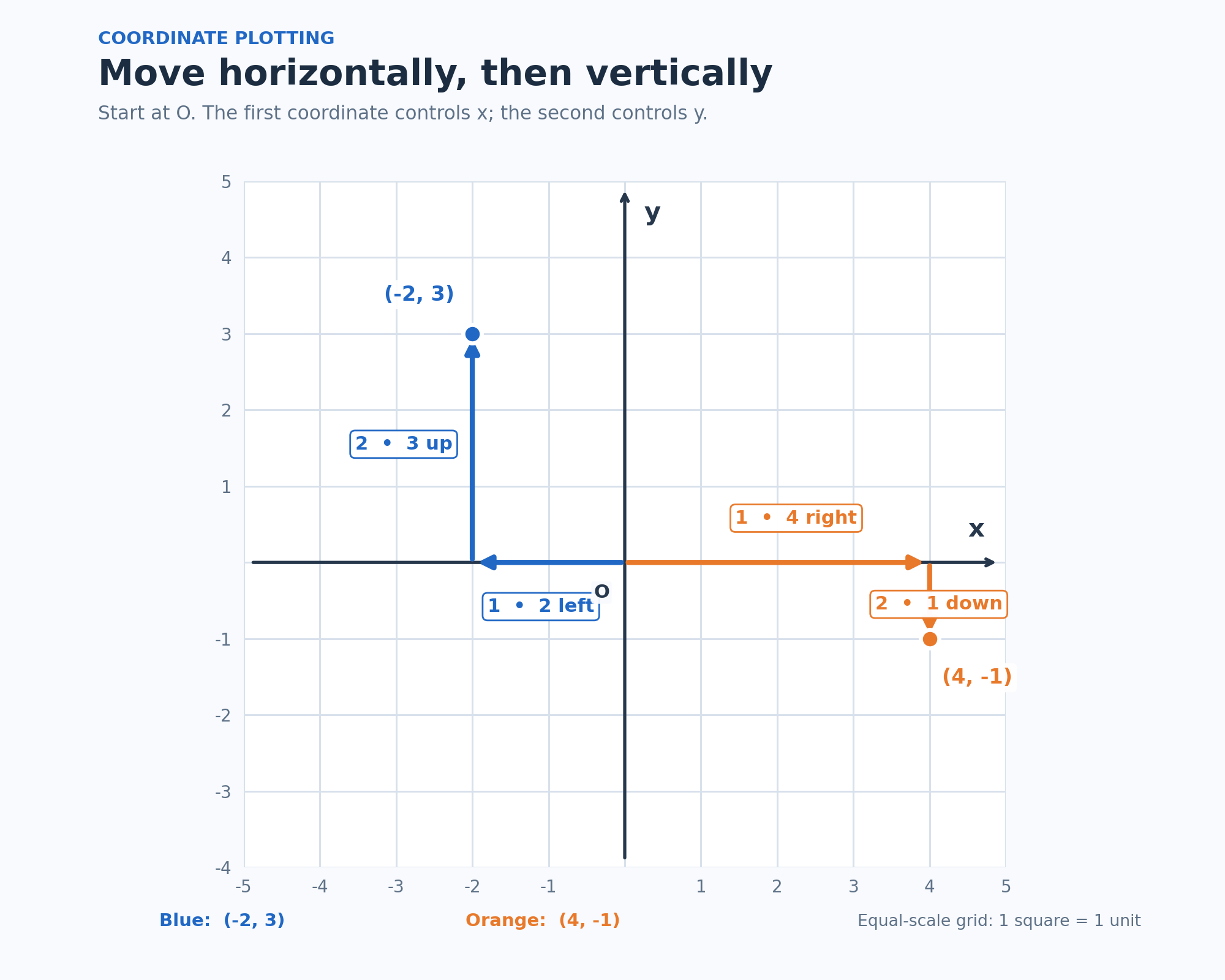
Always inspect the scale before moving. If one grid square represents 2 units, then a coordinate of is two squares from the origin, not four squares. When the variables have units, label the axes so that the graph shows both the locations and what they represent.
Draw a Line Through Two Points
Once the points are in place, construct the single straight path they determine. Any two distinct points determine one geometric line.
Suppose the points are and . Use the following process:
- Plot both points on the same coordinate plane.
- Place a straightedge or line tool so that it passes through both points.
- Draw one straight path through the points without bending or changing direction.
You can use slope as a check, even though you do not need to calculate it before drawing:
The value confirms that the line rises 2 units for every 1 unit it moves to the right. A curved path or a path with a corner would not represent a linear function.
For a graph written as , the two points should have different -coordinates. Two distinct points with the same -coordinate form a vertical line, which is a geometric line but not a function of .
Show the Relevant Visible Segment
A mathematical line continues forever, but a graphing canvas shows only a finite portion. The visible segment is the part of the line that lies inside the displayed graphing window or the allowed domain.
| Given information | How far to draw |
|---|---|
| No restricted domain | Extend the line through both points until it reaches the visible window's boundaries. |
| A domain such as | Draw only the portion whose inputs are in that interval. |
| A real-world starting and ending time | Stop at the meaningful endpoints, even if the mathematical line could continue farther. |
The visible segment can be longer than the distance between the two provided points. Do not stop immediately after connecting those points if the task asks for the line across the visible interval.
Build a Graph from a Value Table
Now combine the earlier skills using the four pairs created from the table. A reliable construction follows this sequence:
- Read across every row and write each ordered pair.
- Plot every point using the axis labels and scale.
- Check that the points align along one straight path.
- Draw one straight line through the points.
- Extend the line across the required visible interval or stop at the allowed domain.
- Verify that each table point still lies on the line.
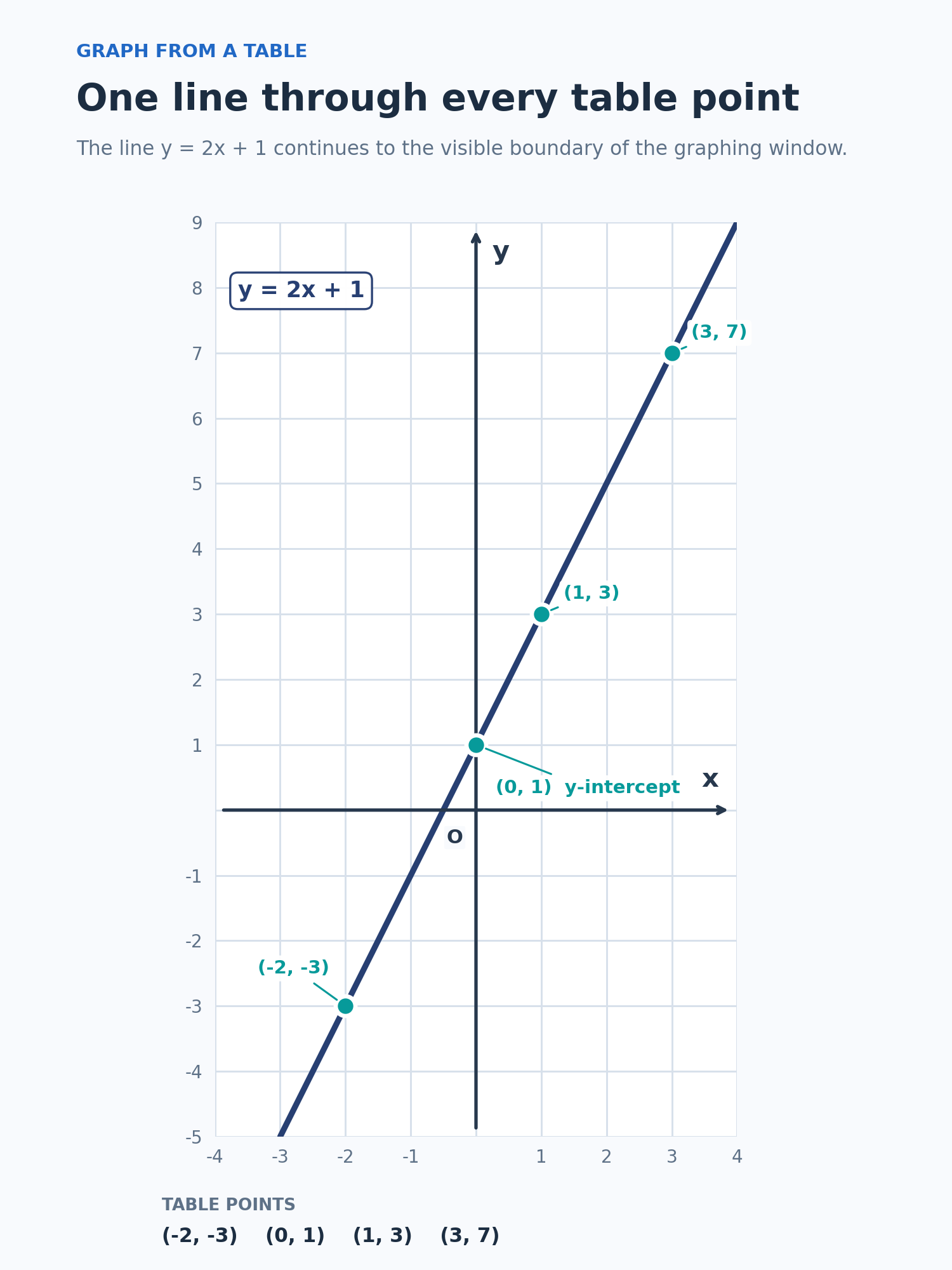
The points in this example follow the rule . For instance, the row with gives
so the point is on the graph. The row with gives , which also provides a quick check on where the line meets the -axis.
If one point appears to miss the line, do not bend the line to include it. First recheck the table row, the order of the coordinates, the axis scale, and the plotted location.
Verify a Line in Context
A graph can point upward and still be incorrect. To verify a seeded line, compare its output with the table for every listed input.
Suppose a worker's earnings include a starting amount and hourly pay. Let represent hours worked and represent earnings in dollars.
| Time (hours) | Recorded earnings (dollars) | Value from | Match? |
|---|---|---|---|
| Yes | |||
| Yes | |||
| Yes | |||
| Yes |
Every listed pair matches the line , so the graph represents the complete table over the domain . A different line, such as , would also rise, but it predicts dollars when instead of the listed dollars. Its direction is reasonable, but it does not represent every pair.
Avoid Common Graphing Errors
Use this table as a final review before constructing a graph.
| Common error | Better approach |
|---|---|
| Reversing as | Put the input first and the output second. |
| Pairing values from different rows | Read across one row at a time. |
| Ignoring negative signs or axis scales | Check the labels before placing each point. |
| Moving to the vertical coordinate before locating | Move horizontally first, then vertically. |
| Drawing a curve or a bent path | Use one straight line for a linear function. |
| Stopping at the two given points | Extend through the required visible interval. |
| Assuming any upward line is correct | Check the output for every listed input. |
| Extending a contextual graph outside its domain | Follow the allowed input values and meaningful endpoints. |
Conclusion and Next Steps
To construct a linear graph, keep each table row together as an ordered pair, place the input on the horizontal axis and the output on the vertical axis, and draw one straight segment through the required points. Two distinct points determine the path, while additional rows provide a check that the graph represents the whole table. The segment must cover the visible graphing interval or the model's allowed domain.
In the practice section, you will begin by matching table rows to their points. You will then construct a visible line from two points, build one from a table, and check a travel or earnings graph one pair at a time. Keep the coordinate order and the relevant interval in view as you work.
