Graphing Linear Equations

Graphing Linear Equations | CodeSignal Learn

Introduction

y

See An Equation as a Graphing Plan

x

Read Slope-Intercept Form

y

Graph From Slope-Intercept Form

y=mx+b

Choose An Efficient Graphing Method

y=-3x+2

Graph A Standard-Form Equation With Intercepts

Ax+By=C.

Check The Line And The Visible Interval

(0,b)

Avoid Common Graphing Errors

b

Conclusion and Next Steps

y=mx+b

Previous Lesson

Join the 1M+ learners on CodeSignal

Be a part of our community of 1M+ users who develop and demonstrate their skills on CodeSignal

An equation may look like a compact rule for calculating an output, but it can also serve as a set of drawing instructions. Once you identify its starting location and its movement, the graph is no longer a guess—you can construct it from the symbols on the page.

You are now in the fifth and final lesson of Linear Graphs, Slope, and Intercepts. Earlier, you learned to recognize linear patterns, measure their constant change, interpret their intercepts, and turn table data into a graph; now you will turn an equation into a graphing plan.

By the end of this lesson, you will be able to:

Read the slope and $y$ -intercept from an equation in slope-intercept form.
Choose an efficient graphing method for a given equation.
Construct a graph from a slope-intercept equation.
Find two distinct axis intercepts from a standard-form equation and graph the line through them.
Extend and check the visible line segment across the required window or domain.

Before you draw, ask two questions: Which point can the equation give you immediately, and how should the line move from that point? For a line that is a function of $x$ , one reliable point plus a constant slope determines the path.

Equation form	Information shown directly	Graphing plan
$y=mx+b$	Slope $m$ and $y$ -intercept $b$	Plot $(0,b)$ , then use the slope to find another point.
$Ax+By=C$ with two distinct intercepts	Points where the line crosses the axes	Set $y=0$ and $x=0$ to find the two intercepts.

Think of $(0,b)$ as a starting address and $m$ as a travel instruction. In standard form, the axis crossings provide two addresses directly, so you can draw the line without calculating its slope first.

These are two routes to the same graph, not two different kinds of line. The best route is the one that produces two clear points with the least unnecessary calculation.

An equation is in slope-intercept form when $y$ is isolated:

y=mx+b

Here, $m$ represents the slope and $b$ represents the $y$ -intercept. Since every point on the $y$ -axis has an $x$ -coordinate of $0$ , the $y$ -intercept is the point $(0,b)$ .

Equation	Slope $m$	$y$ -intercept $b$	First graphing move
$y=4x-3$	$4$	$-3$	Plot $(0,-3)$ ; rise $4$ and run $1$ .
$y=-\frac{1}{2}x+5$	$-\frac{1}{2}$	$5$	Plot $(0,5)$ ; go down $1$ and right $2$ .
$y=7$	$0$	$7$	Plot $(0,7)$ ; draw a horizontal line.

Treat each sign as part of the number. In $y=2x-7$ , the $y$ -intercept is $-7$ , not $7$ ; in $y=-3x+4$ , the slope is $-3$ , so the line decreases as $x$ increases.

If $y$ is not isolated, simplify the equation first by performing the same operation on every term. For example,

2y=6x-8

becomes

y=3x-4.

Now the slope is $3$ and the $y$ -intercept is $-4$ , so the equation is ready for graphing.

You already know how to place ordered pairs and draw a straight path through them. The new skill is using the equation to generate the points, so follow this construction routine:

Rewrite the equation as $y=mx+b$ .
Identify the slope $m$ and $y$ -intercept $b$ .
Plot the point $(0,b)$ .
Use the slope as $\frac{\text{rise}}{\text{run}}$ to locate another point.
Draw one straight line through the points and extend it across the required graphing window or domain.

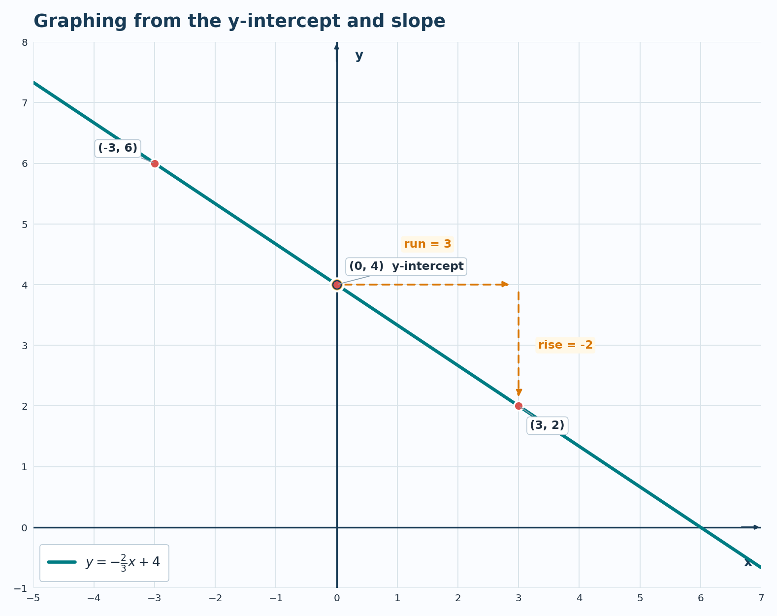
Consider the equation

y=-\frac{2}{3}x+4.

The $y$ -intercept is $4$ , so begin at $(0,4)$ . The slope is $-\frac{2}{3}$ , so one convenient movement is right $3$ units and down $2$ units:

(0,4)\longrightarrow(3,2)

Moving left $3$ units and up $2$ units is also valid, producing the point $(-3,6)$ .

Graph of a line using the y-intercept and a slope movement of right 3 and down 2

A negative slope describes the line's direction as $x$ increases; it does not mean that every coordinate is negative. The line can pass through positive, negative, or zero coordinates while still having a negative slope.

The same graphing plan appears in pricing models. Suppose $P=2.50d+4$ represents the price $P$ , in dollars, of a ride covering $d$ miles. The point $(0,4)$ represents a starting fee, and the slope $2.50$ means that the price increases by $2.50$ dollars per mile.

For a two-mile ride,

P(2)=2.50(2)+4=9.

Therefore, $(2,9)$ is another point on the graph. Because a negative distance is not meaningful in this context, use only the portion of the graph where $d\ge0$ .

Now that you have seen how slope-intercept form provides a starting point and a direction, inspect an equation before doing unnecessary algebra. The quickest method is the one that gives you two easy, distinct points.

Equation situation	Efficient first move	Why
$y=-3x+2$	Plot the $y$ -intercept and use the slope.	Both $m$ and $b$ are already visible.
$2x+5y=10$	Find the axis intercepts.	Setting one variable to zero gives $(5,0)$ and $(0,2)$ .
$4y=8x-12$	Divide by $4$ , then use slope-intercept form.	The equation quickly becomes $y=2x-3$ .

If both methods are reasonable, choose the one that keeps the arithmetic exact and produces points that fit the visible graphing window. Either valid method must produce the same line.

A linear equation is commonly written in standard form as

Ax+By=C.

An $x$ -intercept lies on the $x$ -axis, so its $y$ -coordinate is $0$ . A $y$ -intercept lies on the $y$ -axis, so its $x$ -coordinate is $0$ .

For the two-distinct-intercept method, assume $A\ne0$ , $B\ne0$ , and $C\ne0$ .

Intercept	Coordinate to set to zero	Resulting equation	Point
$x$ -intercept	$y=0$	$Ax=C$ , so $x=\frac{C}{A}$	$\left(\frac{C}{A},0\right)$
$y$ -intercept	$x=0$	$By=C$ , so $y=\frac{C}{B}$	$\left(0,\frac{C}{B}\right)$

Because two distinct points determine a line, you do not need to calculate the slope before drawing it.

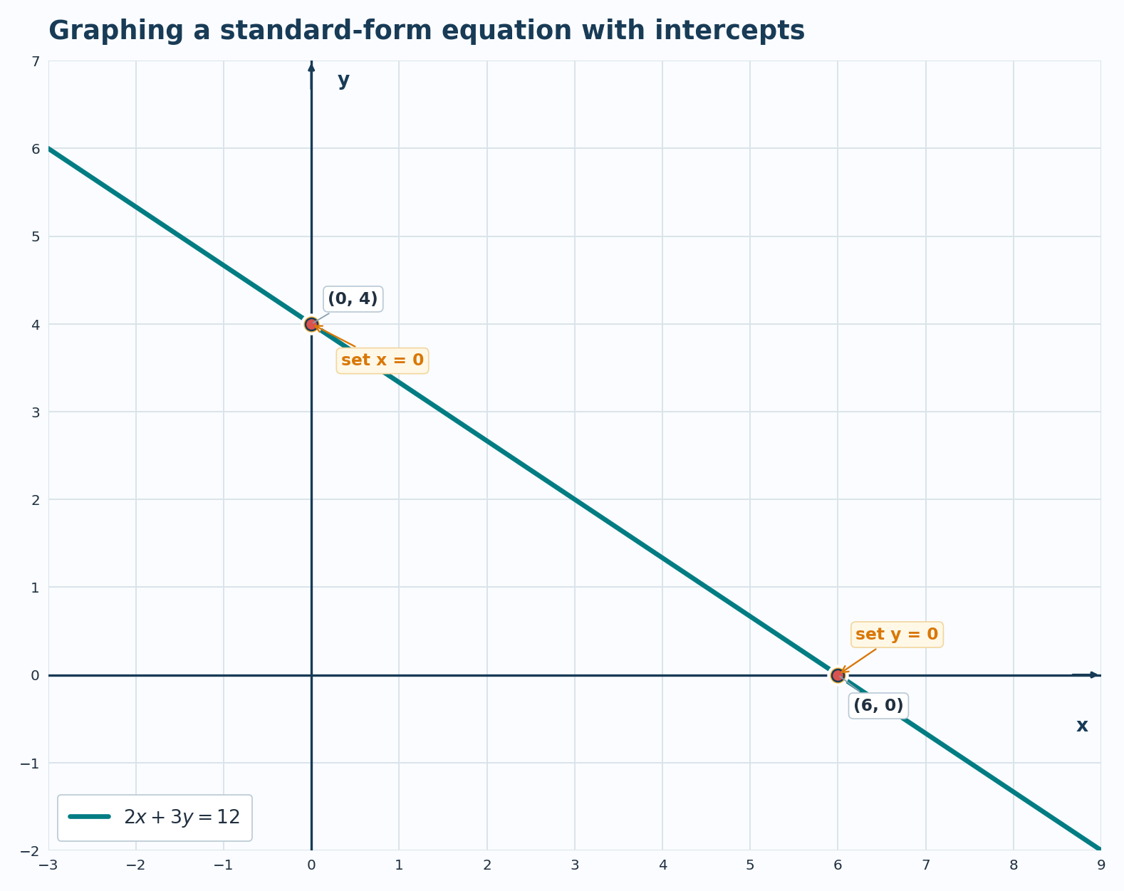
Consider

2x+3y=12.

To find the $x$ -intercept, set $y=0$ :

2x+3(0)=12 \qquad\Longrightarrow\qquad 2x=12 \qquad\Longrightarrow\qquad x=6.

Therefore, the $x$ -intercept is $(6,0)$ .

To find the $y$ -intercept, set $x=0$ :

2(0)+3y=12 \qquad\Longrightarrow\qquad 3y=12 \qquad\Longrightarrow\qquad y=4.

Therefore, the $y$ -intercept is $(0,4)$ . Construct the graph as follows:

Plot $(6,0)$ on the $x$ -axis.
Plot $(0,4)$ on the $y$ -axis.
Draw one straight line through both points.
Extend the line across the required visible window or domain.

Graph of the standard-form equation through the intercepts at 6 comma 0 and 0 comma 4

As a check, isolate $y$ in the original equation:

3y=-2x+12 \qquad\Longrightarrow\qquad y=-\frac{2}{3}x+4.

This confirms that the line has slope $-\frac{2}{3}$ and $y$ -intercept $(0,4)$ , matching the two points you found.

The intercept method is designed for equations with two distinct intercepts. If $C=0$ , both axis calculations produce $(0,0)$ , so you need another point; if $B=0$ with $A\ne0$ , the equation describes a vertical line, and if $A=0$ with $B\ne0$ , it describes a horizontal line.

Your graph is complete only when the plotted points, the equation, and the displayed interval agree. Before you submit it, test the original equation rather than relying only on whether the line looks correct.

Check	What should be true?
Slope-intercept starting point	The line passes through $(0,b)$ .
Slope movement	The change in $y$ matches the stated rise for the chosen run.
Standard-form intercepts	Both calculated intercepts satisfy the original equation.
Window or domain	The visible segment covers the required interval and stops at any stated endpoint.

For the equation $2x+3y=12$ , substitute both intercepts:

2(6)+3(0)=12 \qquad\text{and}\qquad 2(0)+3(4)=12.

Both calculations are true, so both points belong to the line. As in the previous lesson, extend a mathematical line to the graphing window's boundaries unless the problem gives a restricted domain; in a real-world model, stop where the quantities or time period stop making sense.

Most graphing mistakes happen while extracting points, before the line is drawn. Use this table as a final review.

Common error	Better approach
Treating $b$ as the $x$ -coordinate	Plot the $y$ -intercept as $(0,b)$ .
Dropping a negative sign	Keep the sign in both the slope and the intercept.
Reading $-\frac{2}{3}$ as up $2$ and right $3$	Move down $2$ and right $3$ , or move up $2$ and left $3$ .
Finding the $x$ -intercept by setting $x=0$	Set $y=0$ for the $x$ -intercept.
Finding the $y$ -intercept by setting $y=0$	Set $x=0$ for the $y$ -intercept.
Treating the same intercept twice as two points	If both calculations give $(0,0)$ , find another point.
Stopping immediately after plotting two points	Extend the straight line across the required window or domain.
Extending a contextual graph beyond meaningful inputs	Follow the stated domain, such as $d\ge0$ .

An equation can be a complete graphing plan: in $y=mx+b$ , the point $(0,b)$ supplies the location and $m$ supplies the direction; in $Ax+By=C$ with two distinct intercepts, setting one coordinate to zero supplies two axis points. After you plot those points, draw the straight visible segment across the required window or domain and verify it with the original equation.

In the practice section, you will first read slope-intercept equations and choose the more direct method, then construct graphs from both forms. Keep the signs, coordinate order, and endpoint limits visible while you work.