In the previous lesson, you learned how to evaluate a classification model using the confusion matrix and classification report. These tools helped you identify patterns of underfitting or overfitting. Now it’s time to move from diagnosis to fixing. One of the most powerful tools for improving model performance is regularization — a technique that helps control model complexity and improve generalization. In this lesson, you’ll learn how to apply L2 regularization to logistic regression and use the C parameter to find the right balance between underfitting and overfitting.

In real-world applications like spam detection or medical diagnosis, tuning this parameter carefully can dramatically improve the model’s ability to generalize and avoid costly errors.

In scikit-learn’s LogisticRegression, regularization is enabled by default, and the strength of regularization is controlled by the C parameter. One common misconception is that a larger C means stronger regularization — but it’s actually the opposite.

• Smaller C = Stronger regularization → simpler model
• Larger C = Weaker regularization → more flexible model

L2 regularization works by adding a penalty to the loss function that discourages large coefficient values. The result is a model that favors simpler explanations and is less likely to overfit the training data.

Let’s train multiple logistic regression models using different values of C, and observe how regularization strength affects model performance.

• np.logspace(-4, 4, 10) creates 10 values between 0.0001 (10^-4) and 10000 (10^4), spaced evenly on a logarithmic scale. This helps you explore a wide range of regularization strengths.
• solver='liblinear' specifies the algorithm used to fit the model. 'liblinear' is a good default for small datasets and supports L2 regularization.

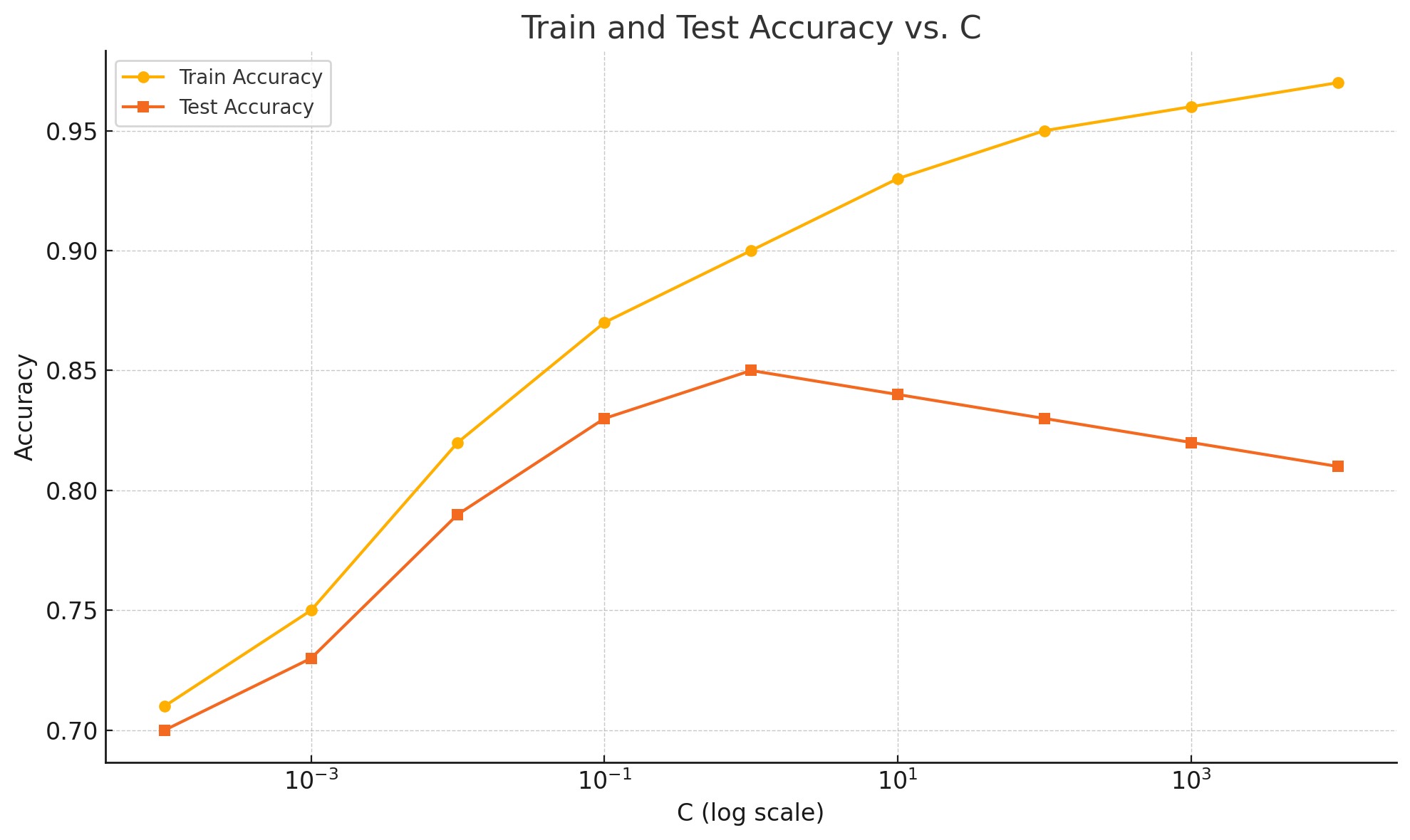
This plot shows how training and test accuracy change as you vary the C parameter (on a logarithmic scale). Notice how test accuracy peaks and then declines as regularization weakens, while training accuracy keeps increasing. This visual makes it easier to spot the "sweet spot" for C.

This table shows how the model behaves as regularization strength changes. A few key patterns stand out:

• At very small C values (e.g., 0.0001), the model is underfitting — it’s too constrained and performs poorly on both train and test sets.
• As C increases (weaker regularization), training accuracy improves and test accuracy initially improves, reaching a peak.
• But at very high C values (e.g., 1000+), the model overfits — training accuracy stays high, but test accuracy declines.

This behavior highlights a classic bias-variance tradeoff. Your goal is to find a C that yields high test accuracy without overfitting.

• Training accuracy always increases with larger C, but that doesn’t mean the model is better.
• Test accuracy improves, then declines — indicating a sweet spot of regularization.
• The best C is usually somewhere in the middle — not too strict, not too flexible.

Try rerunning the model with:

What do you notice about the training and test accuracy now? Does performance improve, or does the model start to memorize the training data?

In this lesson, you explored how L2 regularization in logistic regression helps control model complexity. By tuning the C parameter, you saw firsthand how to move between underfitting and overfitting — and how to find a balance between the two.

In the next lesson, you’ll take these ideas further by switching to decision trees, another model that is highly sensitive to complexity. You’ll learn how to adjust tree depth and observe its impact on generalization performance.