Hello, and welcome to today's exciting lesson! We will delve into the world of neural networks, focusing on a technique called forward propagation, or the data flow from input to output in a neural network.

Neural networks are a variety of machine learning models inspired by the human brain. They draw upon the idea of having neurons interconnected in a net-like structure to process and learn from information, similar to how our brain learns from the data fed into it by our senses. One basic and essential step in how a neural network processes and learns from information is termed forward propagation.

As the name suggests, forward propagation involves moving forward through the network. Each node in the network receives inputs from the nodes in the previous layer, multiplies them by their weights, adds a bias, and then "fires" that through an activation function. The result is then passed on as input to the nodes in the next layer. This process is repeated layer after layer until we reach the output layer, giving us the predicted output.

But what if the predicted output is far from the actual result? That's when backpropagation comes into play. In simple terms, backpropagation is the method used to update the weights of our neural network based on error correction. The less the error, the better our model's predictions.

The entity that quantifies the error between predicted and actual outputs is the loss function. To minimize this loss and hence the prediction error, we use optimization algorithms like gradient descent. In this lesson, we focus on understanding forward propagation, setting a solid foundation for learning more intricate neural network operations such as backpropagation in future lessons.

Now, let's get our hands on practical implementation. We'll use the built-in iris dataset in R for our demonstration:

We start by loading the iris dataset, which is a classic dataset in statistics and machine learning. For this task, we only consider the first two features: sepal length and sepal width. We also convert the problem into a binary classification problem by selecting only the "setosa" and "versicolor" classes.

Next, we preprocess our data:

Scaling the inputs is a common practice in machine learning, as it helps the model converge faster. Here, we use R's scale() function to standardize the features. We then split the data into training and test sets, with 80% for training and 20% for testing.

With our data ready, let's define our simple neural network architecture:

Our neural network consists of one input layer, one hidden layer with 5 neurons, and one output layer with a single neuron (since this is a binary classification problem). We use the relu activation function in the hidden layer and the sigmoid activation function in the output layer.

Let’s take a moment to understand the role of the activation function in a neural network.

An activation function is a function that takes the output of a neuron (input data dot weights, plus bias) and produces a resultant output that is then used as input for the next layer in the network. The activation function introduces non-linearity into the neuron's output. The Sigmoid activation function, used in our model, compresses the outputs of each neuron to a range between 0 and 1. It's especially useful for models where we have to predict the probability as an output.

Besides sigmoid, other commonly used activation functions include:

• ReLU (Rectified Linear Unit): Outputs zero for negative inputs and the input itself for positive values. It is widely used in hidden layers because it helps neural networks learn complex patterns efficiently.
• Tanh (Hyperbolic Tangent): Squashes input values to the range [-1, 1], making it zero-centered and often preferred over sigmoid in hidden layers.
• Leaky ReLU: Similar to ReLU but allows a small, non-zero output for negative inputs, which helps prevent neurons from becoming inactive.

Each activation function is chosen based on the problem and the layer: sigmoid for binary outputs, tanh for zero-centered hidden layers, and ReLU or Leaky ReLU for efficient training in deep networks.

Forward propagation involves flowing forward in the neural network. It takes the input data, performs a dot product with weights, adds the bias, applies the activation function, and passes the result as the input to the next layer. We repeat this until we get our predicted result at the final output layer.

This entire forward propagation operation is handled behind the scenes when you call the fit() function on your model, as shown below:

By calling the compile() function, we configure the learning process. We use adam as our optimizer and binary_crossentropy as our loss function, which is appropriate for binary classification.

When we fit the model, forward propagation occurs in every epoch of training.

The computed output from forward propagation is compared with the actual output to determine the error/cost. The similarity between the predicted and the actual output is captured by the cost function. The goal in training our model is to find the best set of weights and biases that minimize the cost function:

This value represents the model's loss at the last epoch, indicating how well the model performed during training.

After understanding the key concepts behind the operations of a neural network and their implementation in our model, let's see how our model performs on unseen data:

Here, predict() gives the predicted output probabilities, and we convert them to binary values using a threshold of 0.5. We then calculate the accuracy of our model by comparing the predicted output with the actual output.

Finally, let's visualize the decision boundary learned by our model. We'll create a grid that covers the range of our data, predict the output for each point in the grid, and plot the results:

Output:

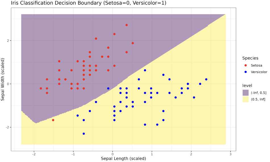
The plot above shows the decision boundary learned by our model. The regions are colored according to the predicted class, and the points represent the actual data points, with color indicating their true class.

That concludes our journey of understanding the basics of the operations within a neural network, focusing on forward propagation and the calculation of the cost function. We used the keras3 package in R to build a simple neural network, making data processing and forward propagation a smoother and more efficient process.

Remember, practical tasks build exceptional skills. In the next lesson, we will tackle more practical tasks designed to test and enhance your understanding of forward propagation, giving you an edge in your machine learning journey. Keep learning and keep improving!