Welcome! In this lesson, we will explore the world of autoencoders — neural networks designed to learn efficient encodings of input data. You’ll become familiar with the autoencoder architecture, focusing on its encoder and decoder components, and how to implement these components using R with the keras3 package. Instead of using image data, we’ll use a generated 2D dataset to clearly visualize how autoencoders perform dimensionality reduction and reconstruction.

Autoencoders are a type of neural network that learns to compress input data into a lower-dimensional space and then reconstruct the original input from this compressed version. They are widely used for tasks such as dimensionality reduction, denoising, and anomaly detection.

Imagine you have a set of points in a 2D space. An autoencoder can learn to represent these points using a single value (1D), and then reconstruct the original 2D points from this compressed representation. This is analogous to creating a simple summary of complex data and then expanding it back to its original form.

The two major components of an autoencoder — the encoder and the decoder — help compress the input data into a latent space and reconstruct the original input from the compressed version.

For this lesson, we’ll generate a synthetic 2D dataset using the mlbench package’s mlbench.2dnormals function. This will allow us to easily visualize the effect of the autoencoder.

Here, we generate 1000 points in 2D space and normalize them so that each feature has mean 0 and standard deviation 1. This normalization step is crucial for training the autoencoder effectively.

Once the data is ready, we move on to implementing the autoencoder components using keras3 in R. The encoder transforms the input data into a latent-space representation (in this case, from 2D to 1D). The decoder then attempts to reconstruct the original 2D input from this compressed 1D representation.

The input shape for the encoder layer is 2, matching the number of features in our data. The encoder compresses the data to a single value, and the decoder reconstructs the original 2D data from this compressed representation.

Now that we've defined the encoder and decoder components, we can compile and train the autoencoder model. The autoencoder will learn to compress the input data into a lower-dimensional space and then reconstruct the original input from this compressed version.

With the autoencoder compiled, we train it using the actual data. This process adjusts the autoencoder's weights to reduce the reconstruction error, improving the model's performance over the training period.

Once the autoencoder is trained, we'll apply it to the data and visualize its effectiveness in reconstructing the input.

We can cross-verify the autoencoder's performance by visualizing a set of actual data points and their reconstructed versions generated by the autoencoder. Here is an example using ggplot2:

Output:

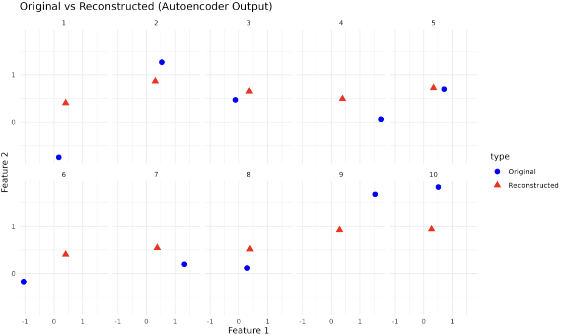
In the above code, we display the original data points and their reconstructed versions side by side for a sample of 10 points. The reconstructed points should be close to the original points, indicating that the autoencoder has learned to compress and reconstruct the input data effectively.

One of the major applications of an autoencoder is dimensionality reduction. By extracting the encoding layers, you can transform the input features into a lower-dimensional space, making it easier to visualize and process.

Since we've already trained our autoencoder model, the encoder will have learned to compress the input data effectively. We can use this learned knowledge to transform our 2-dimensional data into a 1-dimensional encoded space.

Now, encoded_data will be a new representation of our original input data but in the latent space as defined by our encoder. This action is similar to how Principal Component Analysis (PCA) compresses original data into a lower-dimensional space. However, unlike PCA, the encoder, as part of the autoencoder, can capture complex, non-linear relationships, making it a powerful tool for dimensionality reduction.

This compressed representation can be beneficial for various tasks, like feature reduction, data visualization, or even for training other machine learning models, where the fewer number of features can result in less computation.

We've successfully discovered the architecture behind autoencoders, implemented them using R and keras3, compiled and trained our model, and visualized the effectiveness of our autoencoder in reconstructing generated data. Next up, let's exercise to solidify these concepts! Keep practicing, and happy coding!