Welcome to our introduction to Density-Based Clustering and the DBSCAN (Density-Based Spatial Clustering of Applications with Noise) algorithm! Clustering techniques group data based on given measures, with traditional techniques like K-Means focusing on distances between data points. However, Density-Based Clustering seeks areas of high density separated by areas of low density, making it adaptive to a variety of cluster shapes and sizes.

Today, we'll look into DBSCAN's workings and apply it using R. By the end, you'll be proficient in Density-Based Clustering and ready to use DBSCAN on a real-world clustering problem.

DBSCAN is a density-based clustering algorithm that groups together points based on their density. It has two main parameters: eps (epsilon) and MinPts. Here's a brief overview of the algorithm:

1. Initialize: Assign each point a label of 0 (unvisited) and create an empty list of clusters.
2. Iterate over points: For each point, check if it is visited. If not, mark it as visited and find its neighbors within eps distance.
3. Expand clusters: If a point has more than MinPts neighbors, it is a core point. Expand the cluster by adding all reachable points to the cluster.
4. Repeat: Continue until all points are visited.

DBSCAN classifies points into three categories: core points, border points, and noise points. Core points have at least MinPts neighbors within eps distance, border points are within eps distance of a core point, and noise points are neither core nor border points.

Selecting a suitable eps value is crucial for DBSCAN's performance. If eps is too small, many points will be labeled as noise; if it's too large, clusters may merge and lose their distinctiveness. A common approach to choosing eps is to plot the distances to each point's k-th nearest neighbor (where k = MinPts), sorted in ascending order. The "elbow" or point of maximum curvature in this plot often suggests a good eps value. This is known as the k-distance plot method. Experimenting with different eps values and visually inspecting the clustering results can also help in fine-tuning this parameter.

To demonstrate clustering with DBSCAN, we'll first generate some synthetic data using the mvrnorm function from the MASS package. This function generates samples from a multivariate normal distribution, which is perfect for forming distinct "blobs," or clusters, of data.

Next, we'll implement the DBSCAN algorithm itself, along with some necessary helper functions. Specifically, we'll create a distance function, a function to perform a region query, and a function to grow a cluster.

To implement DBSCAN, we first need to calculate the distance between points. For this, we'll use the Euclidean distance, which forms the basis for many machine learning algorithms. The formula for Euclidean distance between two points x and y in a 2D space is:

The region_query function returns all points within a given radius eps from a point P. This helps DBSCAN identify densely populated areas.

The grow_cluster function expands discovered clusters by checking the eps neighbors and including those that meet the MinPts condition.

Next, we will use our helper functions as building blocks for the DBSCAN implementation.

Finally, we apply DBSCAN to our dataset with defined eps and MinPts.

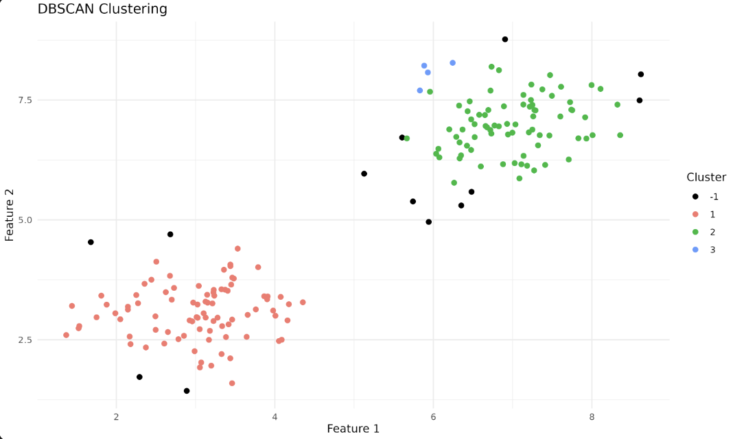
We represent grouped and non-grouped (Noise) data points using the ggplot2 library. Here, -1 marks Noise and is colored black.

Each color here represents a different cluster, helping us visualize the result of our DBSCAN run.

In the output plot, each color represents a different cluster identified by DBSCAN. Points labeled as -1 are considered noise points—these are data points that do not belong to any cluster because they do not have enough neighbors within the specified eps distance. In the plot, noise points (-1 cluster) are shown in black, while other colors represent the discovered clusters. This helps you visually distinguish between clustered data and outliers detected by the algorithm.

And we're done! You dove deep into Density-Based Clustering, implemented DBSCAN, and glimpsed the mathematical equations powering DBSCAN. As we move to the next set of exercises, apply DBSCAN to a variety of datasets and experiment with the eps and MinPts parameters to observe their impact. Enjoy exploring clusters!