Welcome! Today, we'll delve deeper into Density-Based Spatial Clustering of Applications with Noise (DBSCAN) parameters. In particular, we'll explore one crucial yet often overlooked parameter — the distance metric, which defines the distance function used in clustering.
Let's start by generating some sample data for our experiment. We'll manually create two crescent-shaped (moon-shaped) clusters, a common example for demonstrating the capabilities of DBSCAN with non-linearly separable data.
This code generates 400 data points forming two crescent-shaped groups. This type of data is often used to illustrate the capabilities of algorithms like DBSCAN that can capture complex cluster shapes.
Before applying DBSCAN, it's important to standardize the features, especially when using distance-based algorithms. Standardization ensures that each feature contributes equally to the distance calculations.
Before we continue, let's quickly revisit what we mean by distance in the context of the DBSCAN algorithm. In DBSCAN, the definition of what makes data points "neighbors" is fundamental to the functioning of this algorithm, and this definition is rooted in our concept of distance.
We mostly use the Euclidean distance for finding neighbors, but other distance metrics can be employed depending on the problem context. Below is a brief reminder of the common distance metrics:
-
Euclidean Distance: The Euclidean distance between points P1: (p1, q1) and P2: (p2, q2) in a 2D space is
, which is based on the Pythagorean theorem.
We'll fit DBSCAN to our standardized data using three popular distances: Euclidean, Manhattan, and Cosine.
First, install and load the required packages if you haven't already:
Now, let's compute the distance matrices and run DBSCAN with the updated eps values:
- The Euclidean metric calculates the straight-line distance between two points.
- The Manhattan metric measures the sum of absolute differences.
- The Cosine metric calculates the cosine of the angle between two points.
Note: When using a precomputed distance matrix, set search = "dist" in the dbscan function.
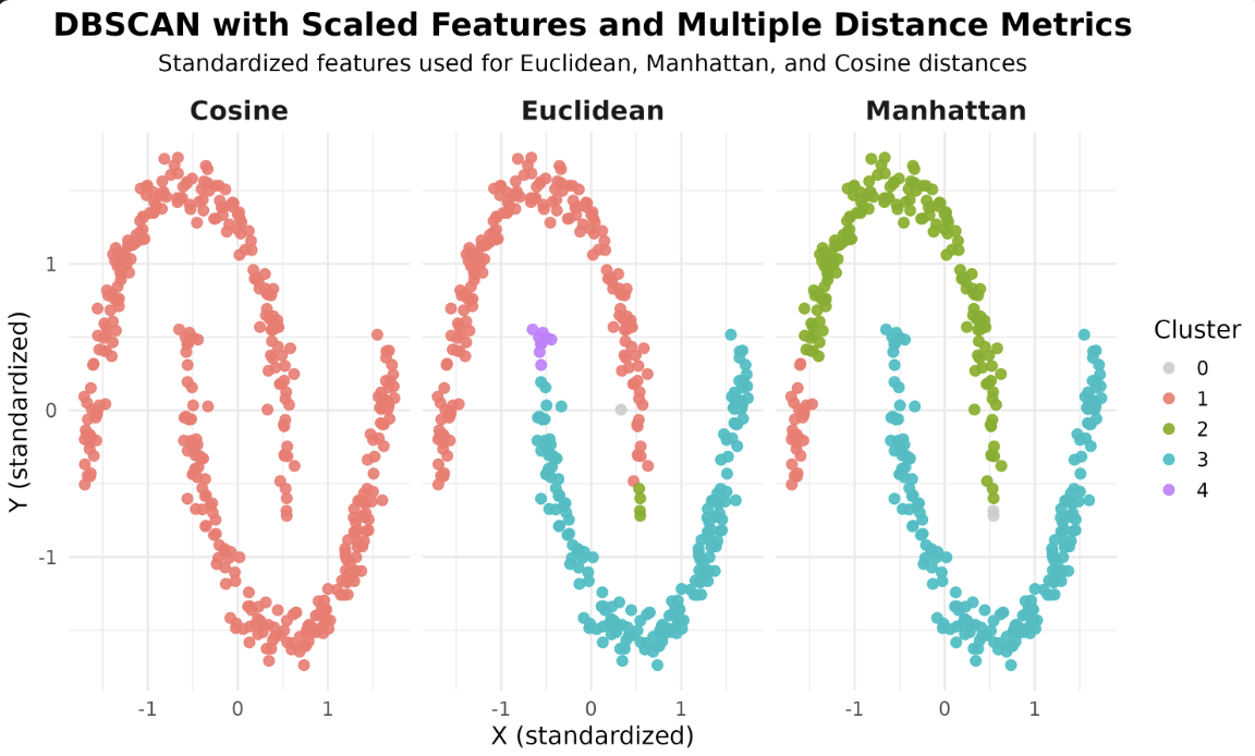
Now that we have our models, let's visualize how different distance metrics affect the DBSCAN results. We'll use ggplot2 to create scatterplots, coloring each point by its assigned cluster and faceting by the distance metric.
In these scatterplots, each point represents a sample, with the color indicating the cluster assigned by DBSCAN. Faceting allows you to compare the effect of each distance metric side by side.
After running the code above, you will see a faceted plot displaying the clustering results for each distance metric. Each facet corresponds to one of the distance metrics: Euclidean, Manhattan, and Cosine.
In R, the dbscan package primarily uses a straightforward approach for neighbor search and does not expose multiple algorithm options like some other libraries. The main way to influence the clustering is by choosing the distance metric, either by specifying it directly or by providing a precomputed distance matrix. For large datasets, consider using the kNN or frNN functions from the dbscan package for efficient neighbor search, but the choice of algorithm is not as configurable as in some other environments.
You've learned how different distance metrics influence the DBSCAN algorithm in R. By experimenting with Euclidean, Manhattan, and Cosine distances, you can observe how the choice of metric affects the clustering results. Keep exploring these parameters and see how they impact your own datasets.
