Welcome back to Deconstructing the Transformer Architecture! This is our third lesson together, and we're making excellent progress building the essential components that power modern language models. In our previous lessons, we explored multi-head attention mechanisms and the feed-forward networks with Add & Norm operations that process information within each Transformer block. Now, we turn to a fundamental challenge that every sequence model must solve: how do we help our model understand the order of elements in a sequence?

Today, we'll tackle Positional Encodings, the ingenious solution that injects sequence order information into Transformer models. Unlike RNNs, which process sequences step by step and naturally encode position through their sequential processing, Transformers process all positions simultaneously through parallel attention operations. This creates both their greatest strength (parallelizability) and a critical challenge: without explicit positional information, attention mechanisms are completely permutation-invariant. We'll implement sinusoidal positional encodings from scratch, visualize their fascinating mathematical patterns, and understand why this elegant solution has become a cornerstone of modern NLP architectures. Let's go!

The self-attention mechanism we've built in previous lessons has a remarkable property that becomes problematic when dealing with sequences: it is permutation-invariant. This means that if we shuffle the order of tokens in our input sequence, the attention mechanism would produce identical outputs for each position, just in the shuffled order. While this property enables efficient parallel processing, it completely ignores the crucial sequential nature of language.

Consider the sentences "The cat sat on the mat" and "Mat the on sat cat the." The words are identical, but their meaning is entirely different due to word order. Without positional information, our attention mechanism cannot distinguish between these fundamentally different sentences. The mathematical reason lies in how attention scores are computed: $\text{Attention}(Q,K,V) = \text{softmax}(\frac{QK^T}{\sqrt{d_k}})V$. Since this computation depends only on the content-based similarity between query and key vectors, permuting the input positions doesn't change the relative relationships between tokens.

Sinusoidal positional encodings solve this problem through an elegant mathematical approach that encodes position using sine and cosine functions with different frequencies. The core insight is to create a unique positional signature for each position that can be added directly to token embeddings without interfering with the learned semantic representations.

The mathematical formulation uses alternating sine and cosine functions across the model dimensions:

Let's implement the complete PositionalEncoding class that creates these sinusoidal patterns:

This initialization creates the foundation for our positional encodings. The position tensor contains values [0, 1, 2, ..., max_len-1] reshaped to enable broadcasting. The div_term computation is the key mathematical insight: it creates the frequency terms that make each dimension unique. By using torch.arange(0, d_model, 2), we generate frequencies for even indices, and the exponential computation creates the geometric progression of frequencies. The use of math.log(10000.0) transforms the original formulation into an exponential form that's computationally stable and efficient.

Now, let's complete the implementation by applying the sine and cosine functions:

Before we can test our positional encodings, we need a TokenEmbedding class that converts token indices to dense vectors:

The TokenEmbedding implementation includes a critical detail often overlooked: the scaling by $\sqrt{d_{model}}$. This scaling ensures that token embeddings and positional encodings have similar magnitudes when added together. Without this scaling, either the token embeddings would dominate (if they're much larger) or the positional encodings would dominate (if token embeddings are too small), both scenarios preventing effective learning of both semantic and positional information. Xavier uniform initialization provides stable starting weights that promote healthy gradient flow during training.

Let's create the complete testing pipeline that generates the expected output and visualization:

This testing pipeline demonstrates the complete workflow from token indices to position-aware embeddings. When we run our complete implementation, we get the following output, which confirms our positional encodings are working correctly:

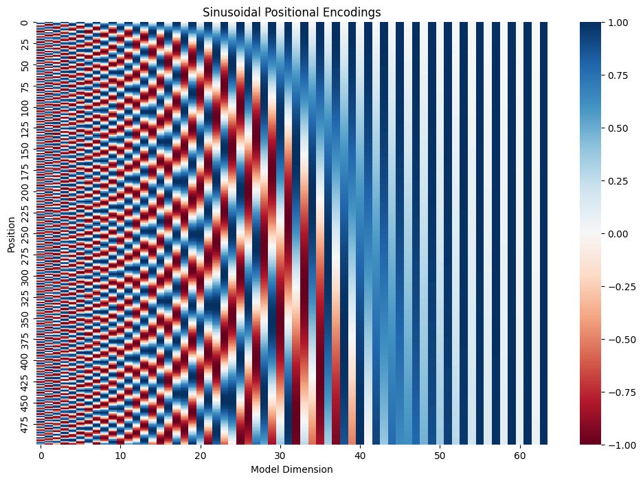
The heatmap reveals the elegant mathematical structure: rows represent token positions, and columns represent model dimensions. Leftmost channels oscillate rapidly with high-frequency patterns, while rightmost channels show nearly constant values, creating a spectrum from fine-grained to coarse-grained positional information. These results demonstrate several key properties: the value range [-1.0000, 1.0000] confirms that our sine and cosine functions are properly bounded, preventing positional encodings from overwhelming token embeddings. The shape preservation across all transformations shows that our implementation maintains dimensional consistency throughout the pipeline. Most importantly, the change in embedding statistics (from mean -0.0141 to 0.4499) indicates that positional information has been successfully integrated with token representations.

We've successfully implemented sinusoidal positional encodings, the elegant mathematical solution that gives Transformers their understanding of sequence order! Our implementation demonstrates how sine and cosine functions with carefully chosen frequencies create unique positional signatures that can extend to sequences longer than those seen during training. The visualization reveals the beautiful mathematical structure, where high-frequency components capture fine-grained positional differences while low-frequency components encode broader positional relationships.

With positional encodings complete, we now have all the core components needed to build a complete Transformer architecture: multi-head attention for relationship modeling, feed-forward networks for non-linear processing, Add & Norm for training stability, and positional encodings for sequence order awareness. In our next lesson, we'll begin assembling these components into complete encoder and decoder layers, bringing us closer to understanding how these individual pieces work together to create the powerful language models that have transformed NLP. Time to practice with these positional encodings!