Welcome back to Compound Event Probability! You have reached lesson five of five — the final lesson in this course. Congratulations on making it this far! Over the previous four lessons, we built a complete toolkit for organizing and counting outcomes of compound events: we identified what makes an event compound, used organized lists with the fix-and-cycle technique, arranged outcomes in two-way tables, and constructed tree diagrams that extend to three or more stages.

Each of those tools helped us find theoretical probabilities by carefully listing every equally likely outcome. But what happens when listing every outcome is too complex, or when the real-world situation does not give us perfectly equal probabilities? In this lesson, we explore a powerful alternative: simulation. You will learn how to design a simulation that mirrors a compound event, run it over many trials, estimate the event's probability from the results, and compare that estimate to the theoretical value when one is available.

As you may recall from the earlier course on experimental probability, we can estimate how likely an event is by repeating an experiment many times and tracking how often the event occurs. That ratio of favorable trials to total trials is called the relative frequency, and it tends to settle closer and closer to the true probability as the number of trials grows.

Simulation applies this same idea to compound events. Instead of physically acting out every scenario, we use a random device — such as a coin, a die, a spinner, or a computer random-number generator — to imitate each stage of the event. By repeating the process many times and recording the results, we build up data that lets us estimate the probability without listing every possible outcome by hand.

Think of simulation as a shortcut that trades perfect precision for practical convenience. A tree diagram with five stages might produce hundreds of paths to trace, but a simulation can churn through thousands of trials quickly and still land close to the true answer.

The most important step in designing a simulation is picking a random device that matches the probability structure of each stage. The device must have the same number of equally likely options as the stage it represents.

Here are some common matchups:

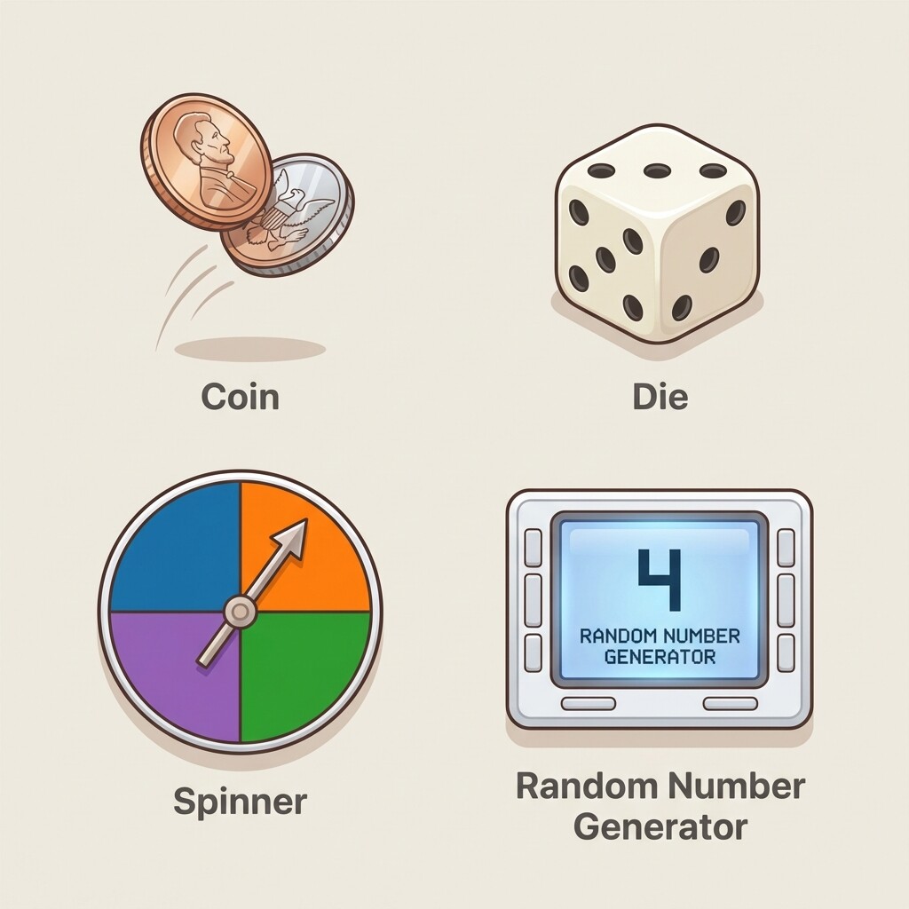
The key rule is straightforward: count the equally likely options at each stage, then choose a device with the same count. If Stage 1 has 3 options and Stage 2 has 2 options, you might roll a die for Stage 1 (mapping the results 1–2, 3–4, and 5–6 to the three options) and flip a coin for Stage 2. As long as each device gives every option the same chance of being selected, the simulation accurately mirrors the original event.

Once the random device is chosen, we need to define four components before running a single trial. Think of this as the blueprint for the simulation:

1. Random device for each stage: What tool represents each stage, and how do outcomes map to the real event? For instance, "Roll a die: 1–2 = Rain, 3–4 = Cloudy, 5–6 = Sunny."
2. What one trial consists of: A trial must walk through every stage of the compound event once. If the event has two stages, one trial involves using the device twice (once per stage) and recording the combined result.
3. What counts as a favorable outcome: State the specific combination or condition we are looking for. For example, "a trial is favorable if the first stage result is Rain and the second stage result is Late."
4. How many trials to run: More trials give a more stable estimate. A common starting point is 50 to 100 trials for a classroom simulation, though real-world applications often use thousands or more.

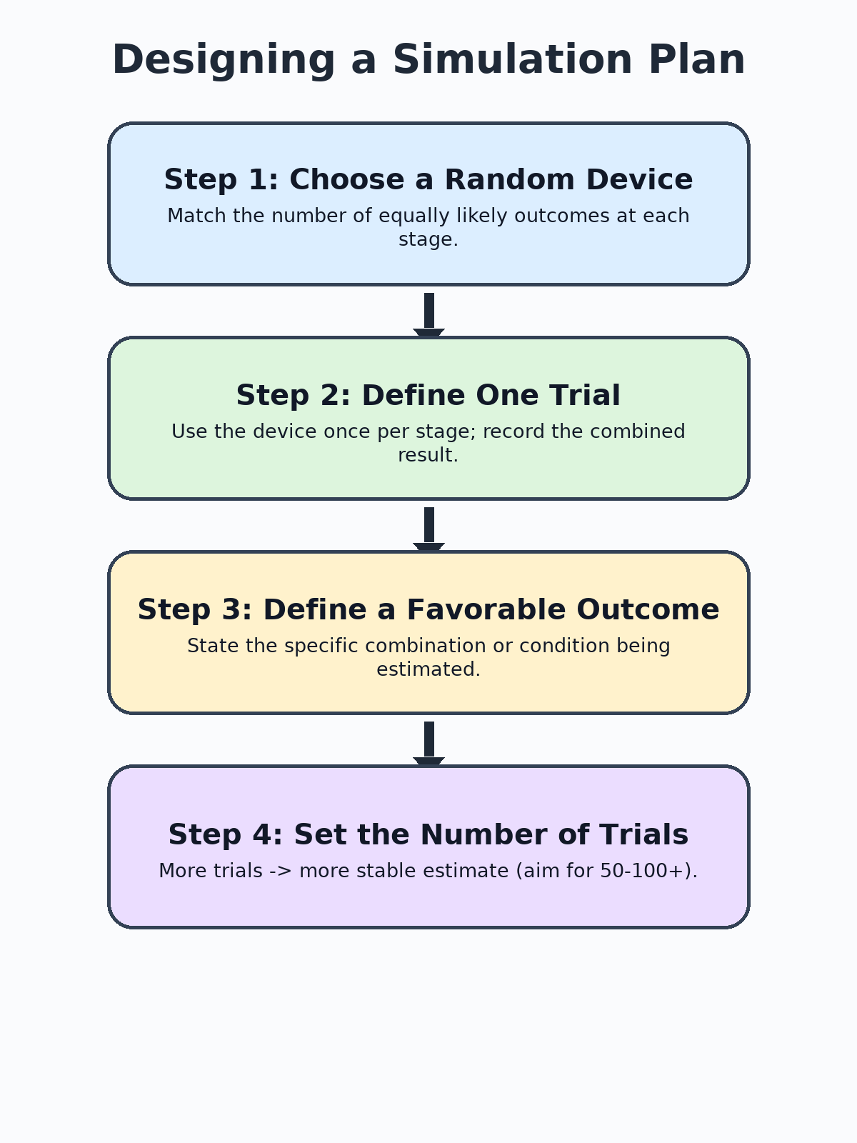
Writing out this plan before collecting data keeps the simulation organized and repeatable. Skipping any one of these components usually leads to confusion midway through, so take a moment to set all four in place first.

After running all the trials, we calculate the estimated probability using the relative-frequency formula you practiced in an earlier course:

$$P_{\text{simulated}}(\text{event}) = \frac{\text{number of favorable trials}}{\text{total number of trials}}$$

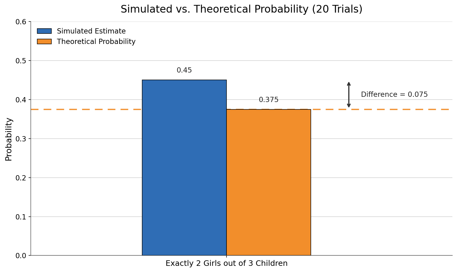
When a theoretical probability is available, we should compare it to our simulation result. For the three-child example, we can list all $2 \times 2 \times 2 = 8$ equally likely outcomes using a tree diagram or organized list: HHH, HHT, HTH, HTT, THH, THT, TTH, TTT. Exactly three of these (HHT, HTH, THH) contain two girls, so:

$$P_{\text{theoretical}}(\text{exactly 2 girls}) = \frac{3}{8} = 0.375$$

Let's design a simulation from scratch for a slightly richer scenario. A bakery offers a free mini-treat promotion: each customer spins a spinner with 3 equal sections (Cookie, Brownie, Muffin) on two separate visits. We want to estimate the probability that a customer gets the same treat on both visits.

Step 1 — Choose the device. Each stage has 3 equally likely options, so we can use a standard die with a simple mapping: 1–2 = Cookie, 3–4 = Brownie, 5–6 = Muffin.

Step 2 — Define one trial. Roll the die twice. Record the treat for each roll using the mapping.

Step 3 — Define a favorable outcome. Both rolls produce the same treat (e.g., Cookie and Cookie).

Step 4 — Set the number of trials. We will run 50 trials.

After running 50 trials, suppose we observe that 15 trials resulted in matching treats:

$$P_{\text{simulated}}(\text{same treat}) = \frac{15}{50} = 0.30$$

In this lesson, we added simulation to our compound-event toolkit. We learned that the foundation of a good simulation is choosing a random device that mirrors the probability structure of each stage. From there, we define what one trial looks like, state what counts as a favorable outcome, decide how many trials to run, and then use the relative-frequency formula to estimate the probability. When a theoretical probability is known, comparing it to the simulated estimate helps us check our work and reinforces that small differences are natural, especially with a modest number of trials.

You have now completed all five lessons in Compound Event Probability — from recognizing compound events, through organized lists, tables, and tree diagrams, all the way to designing your own simulations. Up next are practice exercises where you will choose simulation devices, complete simulation plans, crunch real trial data, and walk through an entire simulation design on your own. Dive in and bring everything you have learned together!