Filtering and Evaluating Model Candidates
Introduction
By the end of previous lesson, you could look at a model identifier and correctly name its family, its provider, and its access route. But knowing that openai/gpt-5.6-luna is OpenAI's GPT family, version 5.6, doesn't tell you whether it's the right choice for the categorization tool you're actually building. The common failure mode here is picking a model because it has the best benchmark score, the flashiest catalog label, or simply the most name recognition — and skipping the harder question of whether it satisfies what your specific application actually demands.
What follows is a repeatable way to answer that question. You'll learn to sort a list of project requirements into what a model must satisfy versus what you'd merely prefer, use that sorted list to eliminate unviable candidates from a model-profile table before testing anything, interpret controlled evaluation results where the model — not the prompt — is the variable that changed, and finally combine that evaluation's evidence with an operational profile covering cost, latency, and rate limits to land on one defensible choice. The habit to build: filter first on hard requirements, gather evidence second, decide last — never let a preference eliminate a candidate, and never let quality alone override a requirement it fails.
Hard Requirements vs. Optimization Tradeoffs
Every project comes with a list of stated conditions, and the first skill is telling two very different kinds apart.
A hard requirement is a condition a model must satisfy or it is disqualified outright, no matter how well it performs otherwise. "Must support image attachments," "customer data must stay in-region," "responses must complete in under 2 seconds" — each of these draws a hard line. Fail it, and the model is out of consideration regardless of any other strength.
An optimization tradeoff is a preference you weigh among the models that already clear every hard requirement. "We'd like to minimize per-message cost" and "faster is better, but there's no strict cutoff" are both tradeoffs — worth optimizing, but not disqualifying on their own.
Here's the part that trips people up: the same dimension can appear in either bucket depending on how it's worded. Latency — how long the model takes to respond — can be a hard requirement ("must respond in under 2 seconds") or a tradeoff ("ideally faster, no fixed cutoff"). Cost can go either way too: "inference must stay below $5,000/month" is a hard requirement, while "prefer lower cost" is a tradeoff — it's the wording that tells you which bucket applies, not the dimension itself. A useful shortcut:
- Signal words for hard requirements: "must," "required," "mandatory," "cannot," "only if."
- Signal words for tradeoffs: "prefer," "ideally," "should minimize where possible."
Take a support-chat project with this requirements list:
- "Must support image attachments from users" — hard requirement (multimodal, meaning the model can work with more than text, such as images).
- "Customer data must stay in-region" — hard requirement (privacy/data-handling).
- "Responses must complete in under 2 seconds" — hard requirement (latency ceiling).
- "We'd like to minimize per-message cost" — tradeoff.
- "Among models meeting that ceiling, faster is preferred" — tradeoff.
Notice that latency shows up twice in this list, once as a hard ceiling and once as an optimization preference among qualifying models — that's exactly the distinction to watch for.
Once a requirement is labeled "hard," it stops being an abstract statement and becomes a filter. Some hard requirements can be checked before evaluation, such as required capabilities or a latency limit; others, such as a minimum task-specific quality score, can only be checked after you run the evaluation. The ones you can check up front apply directly to a model profile table — that's the next move.
Running One Controlled Evaluation Across Candidate Models
This step reuses discipline you already built when comparing Prompt A against Prompt B: freeze every condition except the one thing you're testing, so any difference in results can be attributed to that one variable. Previously, the prompt was the variable and the model was held fixed. Now that flips — the model is the variable, and the prompt, cases, metric, expected answers and run count all stay identical across every candidate you test. Runs still measure reliability within a model, and cases still measure coverage across a range of inputs; neither of those meanings changes just because the model changed.
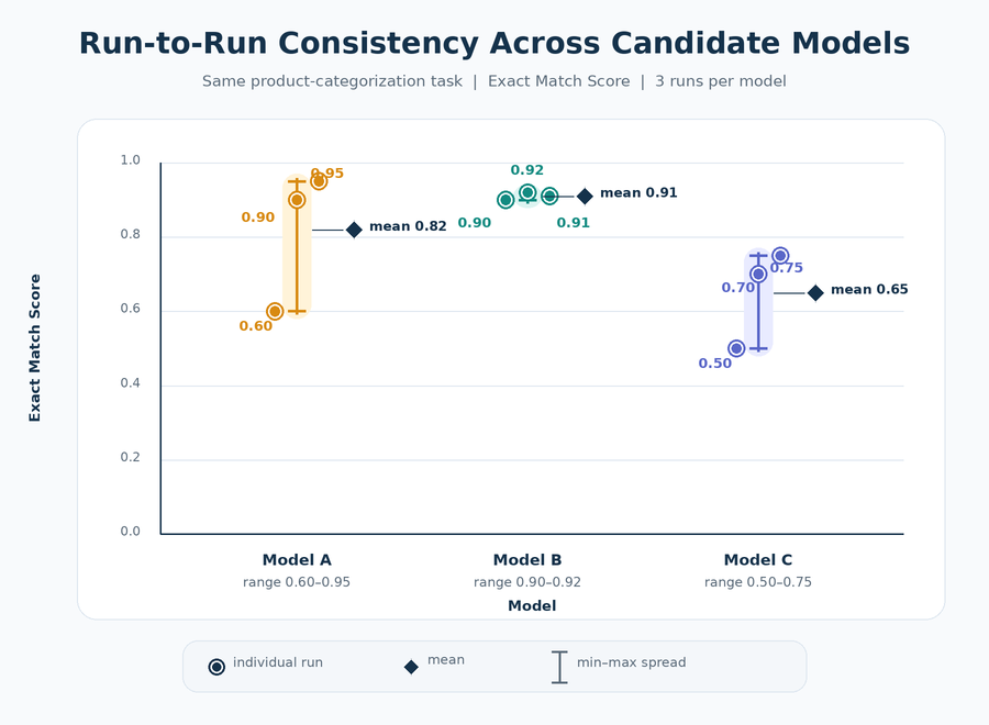
The reason for multiple runs is simple: model outputs can vary from one run to the next, so we run each model several times. If the scores stay close together, that gives us more confidence the model's behavior is consistent.
Picture a product-categorization job. The prompt reads: "Categorize this product listing into exactly one of: Electronics, Home & Kitchen, Apparel, Other." The cases are a fixed set of product descriptions, each with an Expected Answer (a category label). Because categories are short, discrete labels, Exact Match (case-insensitive) is the right metric — you're checking whether the model landed on the correct label exactly, ignoring differences in capitalization, not whether its phrasing was similar. You review 3 runs per model across three allowlisted candidates, A, B, and C, keeping prompt, cases, metric, and run count identical across all three:
| Model | Run 1 | Run 2 | Run 3 | Mean |
|---|---|---|---|---|
| Model A | 0.60 | 0.90 | 0.95 | (0.60+0.90+0.95)/3 = 2.45/3 = 0.82 |
| Model B | 0.90 | 0.92 | 0.91 | (0.90+0.92+0.91)/3 = 2.73/3 = 0.91 |
| Model C | 0.50 | 0.70 | 0.75 | (0.50+0.70+0.75)/3 = 1.95/3 = 0.65 |
These figures are illustrative — a live run against real candidates would produce its own results, not this exact table. Reading it the way you'd read any evaluation Results: Model B has the highest mean and shows more consistent results across these three runs (0.90 to 0.92). Model A's mean (0.82) looks respectable at a glance, but its individual runs span 0.60 to 0.95 — much greater run-to-run variation that counts as a mixed result and is worth flagging even when the mean alone looks fine. Model C trails on both the mean and the spread.
This process produces task-specific quality evidence for each surviving candidate. But notice what the table doesn't tell you: nothing here about cost, response speed under load, or how many requests each model can handle per minute. The highest-scoring model in an evaluation table isn't automatically the right choice once those real-world operating constraints enter the picture.
Combining Quality Evidence with Operational Constraints to Choose
The following diagram demonstrates an example of a model-choosing process.
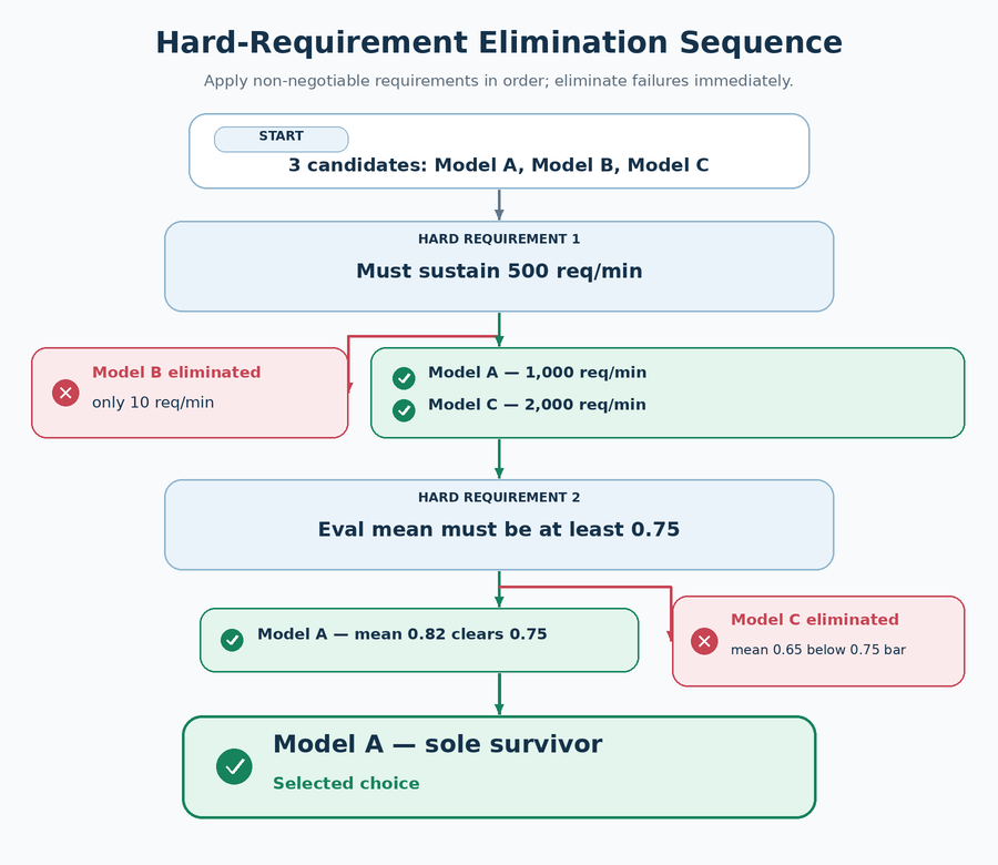
We combine task-quality evidence with operational constraints, applying hard requirements before ranking preferences such as cost.
Model B has the strongest evaluation mean but fails the rate-limit requirement; Model C meets the rate limit but misses the accuracy floor. Model A is the only candidate that clears both gates, though sustained throughput still needs load testing.
Conclusion
The core shift is this: model choice stops being "pick the model with the best reputation or the best single score" and becomes a two-stage discipline. First, classify every stated condition as a hard wall or a soft preference — wording, not the dimension itself, tells you which bucket it belongs in. Second, let only hard walls eliminate candidates; preferences and evaluation scores come into play only among whoever survives.
Carry the pattern forward as Classify → Filter → Evaluate → Decide. Classify each stated requirement as hard or tradeoff. Filter the candidate catalog using hard requirements alone, before reviewing evaluation results. Evaluate candidate performance on your task using controlled evidence — identical prompt, cases, metric, expected answers and run count, with the model as the only variable. Decide by re-applying hard requirements to the operational profile, eliminating anyone who fails, then ranking whoever's left by priority.
The exercises ahead follow this exact sequence: sorting requirement statements into hard requirements and tradeoffs, filtering a profile table for a specific workload, analyzing controlled evaluation results across candidate models, and combining that evaluation's results with an operational table to make the final call. The next unit picks up right where this one ends — examining how much confidence to place in model-evaluation evidence and recognizing when more validation is needed before making a choice.
