Non-Uniform Probability Models

Welcome back to Building Probability Models! You are now on lesson three of five, meaning you have crossed the halfway mark of this course. So far, you have learned how to check whether a probability model is valid and how to build a uniform model for equally likely outcomes. Those skills form a solid foundation for what comes next.

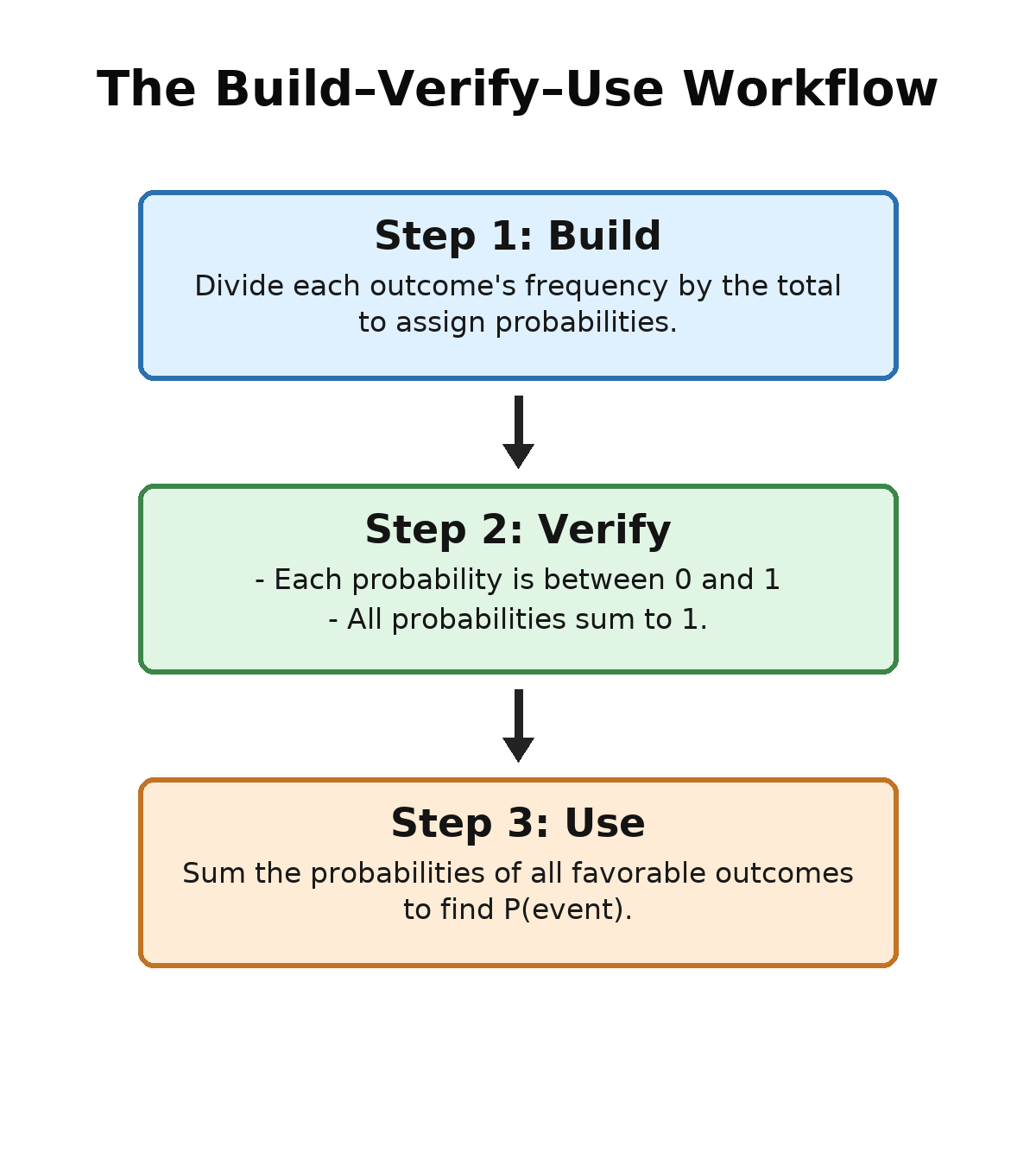
In this lesson, we tackle the kind of situation you will encounter most often in the real world: outcomes that are not equally likely. We will learn how to construct a non-uniform probability model from observed data or known rates, verify it, and use it to find event probabilities. The same build–verify–use workflow you practiced last time still applies, but the way we assign probabilities changes.

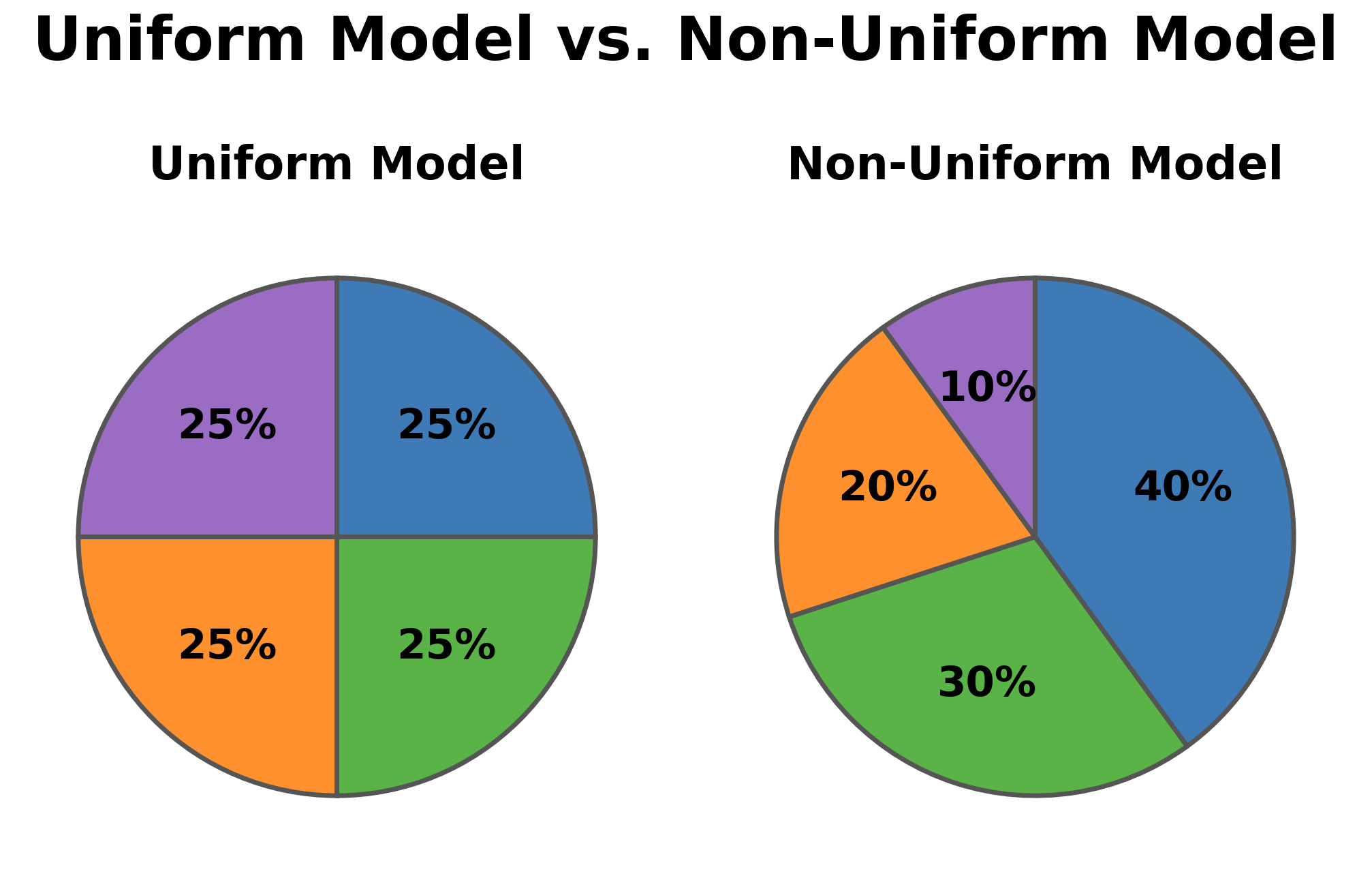
A uniform model gives every outcome the same probability. That works well for fair coins, balanced dice, and random draws. But many everyday situations do not split evenly. Think of a clothing store tracking returns by reason: "wrong size" might account for half of all returns, while "defective item" might be quite rare. Or consider a city's weather patterns, where sunny days could be far more common than snowy ones.

When some outcomes naturally occur more often than others, forcing equal probabilities would misrepresent reality. Instead, we need a model that lets each outcome carry its own weight, and that is exactly what a non-uniform probability model provides.

The most common way to assign unequal probabilities is to use observed data. Earlier in this learning path you saw that relative frequency is a natural estimate of probability. The same idea drives non-uniform model construction: divide each outcome's count by the total number of observations.

Let us see this in action. A bakery tracked its last $200$ muffin orders and recorded the following counts:

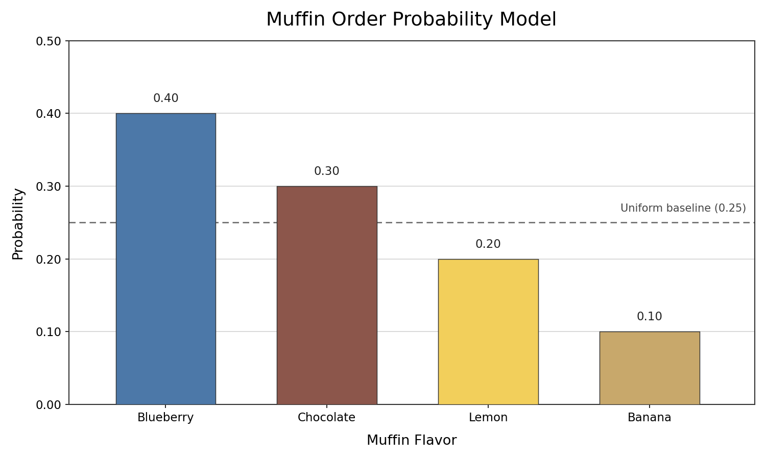
To build the model, we divide each count by the total ($200$):

That table is our non-uniform probability model. Notice that each outcome carries a different probability, reflecting how frequently it was ordered. Blueberry is the most popular, and banana is the least. The data, not an assumption of fairness, drives the model.

It is worth noting that frequency data is not the only source. Sometimes probabilities come from known proportions (for example, a bag filled with $70\%$ red and $30\%$ blue marbles) or historical rates (for example, a factory's published defect rate). The idea is the same in each case: assign each outcome the probability that best reflects its actual likelihood.

Building a model is only useful if the result is valid. Every probability model must still satisfy the two requirements you learned in the first lesson of this course. Let us check them for the bakery model.

Requirement 1 — each probability is between $0$ and $1$: The values $0.40$, $0.30$, $0.20$, and $0.10$ all fall within the range $[0, 1]$. ✓

Requirement 2 — probabilities sum to $1$:

Both checks pass, so this is a valid probability model. When you compute probabilities by dividing each frequency by the same total, the sum is guaranteed to reach $1$ because the individual counts add up to that total. However, verification remains a good habit, especially when probabilities are given to you or when rounding is involved.

Once the model is built and verified, we find event probabilities the same way we did with uniform models: sum the probabilities of all favorable outcomes in the event.

The key difference is that we can no longer use the $\frac{k}{n}$ shortcut from uniform models, because the individual probabilities are not all equal. We must add each favorable outcome's specific probability.

Let us try it with the bakery model. Suppose we want the probability that the next customer orders a fruit-flavored muffin (blueberry, lemon, or banana):

The model estimates a $70\%$ chance the next order is fruit-flavored. Notice how blueberry's larger probability pulls the event probability up. In a uniform model with four flavors, each would contribute $0.25$, and three flavors would give $0.75$. Here, the unequal weights shift the answer to $0.70$, giving a more accurate picture of reality.

Let us practice the full build–verify–use workflow with a fresh scenario. A tech company reviewed its last $400$ support tickets and sorted them by issue type:

Step 1 — Build the model. Divide each count by the total of $400$:

Step 2 — Verify the model. Each probability is between $0$ and $1$. The sum is:

The model is valid. ✓

Step 3 — Find an event probability. What is the probability that the next ticket involves an account or billing issue? The favorable outcomes are Account Access and Billing Question:

There is a $45\%$ chance the next ticket relates to account access or billing. The three-step workflow gives us a clear path from raw data to a meaningful probability, even when outcomes are far from equally likely.

A non-uniform probability model assigns different probabilities to different outcomes, capturing the reality that some results are more common than others. We build these models by dividing each outcome's observed frequency by the total number of observations, though probabilities can also come from known proportions or historical rates. The model is valid as long as every probability falls between $0$ and $1$ and the sum equals $1$. To find the probability of an event, we sum the probabilities of all favorable outcomes, just as we did with uniform models.

Up next, you will put these ideas into practice by building non-uniform models from real-world data, spotting valid models among impostors, and computing event probabilities across a variety of everyday scenarios. Jump in and see how rewarding it is to turn messy, unequal data into a clean and useful probability model!