Welcome to Analyzing Data with Box Plots, the fourth course in this learning path! Over the previous three courses, you have built a solid toolkit: measures of center, measures of spread like the range and IQR, and the ability to read and interpret histograms. Now we are going to explore another powerful visualization that packs a surprising amount of information into a simple graphic.

In this first lesson, we will learn how to read a box plot. By the end, you will be able to look at any box plot and confidently identify its five key values: the minimum, first quartile ($Q_1$), median, third quartile ($Q_3$), and maximum.

As you may recall from earlier courses, when we computed quartiles and the IQR we were working with five important values that together describe a dataset's spread and center:

• Minimum — the smallest value
• $Q_1$ (first quartile) — the value below which 25% of the data falls
• Median — the middle value (50th percentile)
• $Q_3$ (third quartile) — the value below which 75% of the data falls
• Maximum — the largest value

These five numbers are collectively called the . Until now, we calculated them from raw data. A box plot is simply a picture that displays all five of these values at once, making it easy to see center, spread, and overall shape in a single glance.

A box plot sits along a number line (which can be horizontal or vertical). It has three main visual pieces: a box, a line inside the box, and two whiskers. Let's walk through each one.

The box is a rectangle that stretches from $Q_1$ on one side to $Q_3$ on the other. Inside the box, a vertical (or horizontal) line marks the median. Because the box spans from ${}_{}$ to , its width represents the , which covers the middle 50% of the data.

Now that you have seen the big picture, here is a compact reference table you can return to any time you need a reminder of which part maps to which statistic:

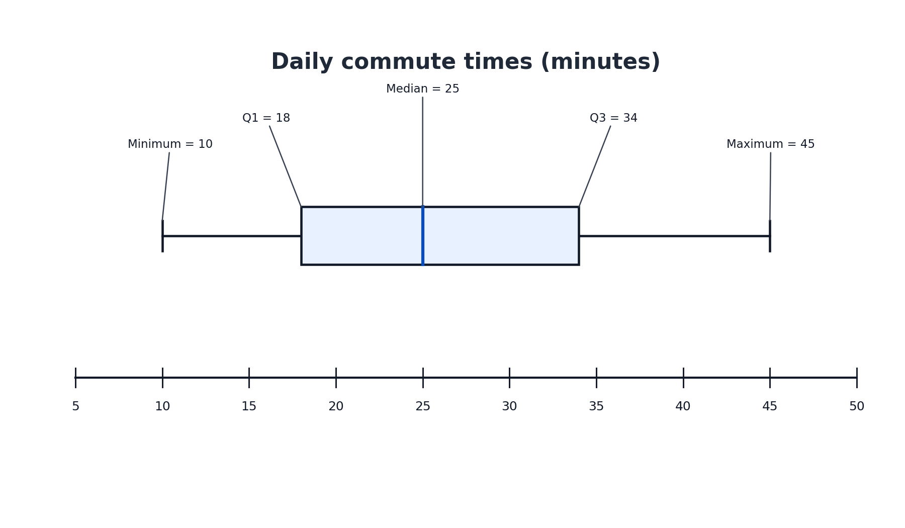
Imagine a horizontal box plot showing daily commute times (in minutes) for a group of employees, placed above a number line that runs from 5 to 50. A plot like this would look as follows:

Working from left to right along the number line, here is what we observe:

1. The left whisker ends at 10. This is the minimum: the shortest commute is 10 minutes.
2. The left edge of the box sits at 18. This is $Q_1$: 25% of commuters have a commute of 18 minutes or less.
3. The line inside the box falls at 25. This is the median: the middle commute time is 25 minutes.
4. The right edge of the box sits at 34. This is $Q_3$: 75% of commuters have a commute of 34 minutes or less.

Reading a box plot is straightforward once you know what to look for, but a few simple habits will help you avoid common mistakes.

• Check the scale. Look at the number line first. Note the units and the spacing between tick marks so you do not misread a value.
• Work from left to right (or bottom to top for vertical plots). Start with the minimum at the whisker tip, then move to $Q_1$, the median, $Q_3$, and finally the maximum. Going in order helps you stay organized.
• Distinguish the median from the box edges. The line inside the box is the median. It is easy to confuse it with the edges, so look carefully at its position relative to and .

In this lesson, we learned that a box plot is a visual display of the five-number summary: minimum, $Q_1$, median, $Q_3$, and maximum. The box captures the middle 50% of the data, the median line marks the center, and the whiskers stretch out to the smallest and largest values. Reading a box plot comes down to matching each visual feature to its spot on the number line.

Up next, you will put these skills to work in a set of hands-on practice tasks where you will identify, label, and read values from box plots. You will start by matching each part of the graphic to its statistical name, then practice reading individual values, and finally extract a complete five-number summary on your own — let's jump in!