In previous work with ray tracers, you've likely used a simple, fixed camera that always looks in the same direction from the same position. While this works for basic scenes, it's quite limiting. Imagine trying to photograph a landscape but being unable to move or turn your camera — you'd miss most of the interesting shots!

A real camera has three fundamental properties: it exists at a specific position in space, it points toward something, and it maintains an orientation (you don't want your photos tilted sideways). In this lesson, we'll build a camera class that gives you full control over these properties, allowing you to position your virtual camera anywhere in your scene and point it at anything you want to render.

By the end of this lesson, you'll understand how to transform high-level camera parameters like "I want to look at this sphere from over here" into the actual rays that trace through your scene. We'll explore how the camera creates its own coordinate system, how the field of view affects what you see, and how all these pieces work together to generate rays for each pixel in your final image.

Let's start with the most intuitive aspects of camera control: where it is and where it's looking. Think about holding a real camera in your hands. You're standing at a specific location (your position), you're pointing the camera at something interesting (your target), and you're holding it level so the horizon isn't tilted (your orientation).

In our ray tracer, we define these three concepts with vectors:

The lookfrom vector specifies where the camera is located in 3D space. In this example, the camera sits at position (3, 3, 2) — three units to the right, three units up, and two units forward from the origin. This is your camera's physical location in the world.

The lookat vector specifies the point in space that the camera is aimed at. Here, we're looking at the point (0, 0, -1), which is slightly behind the origin along the negative z-axis. The camera will orient itself so that this point appears in the center of your rendered image. Think of this as the spot where you're focusing your attention.

The vup vector (short for "view up") defines which direction is "up" from the camera's perspective. In most cases, you'll use (0, 1, 0), which means the positive y-axis points upward. This keeps your camera level with the world. If you changed this to (0, -1, 0), your image would appear upside down, like holding a camera over your head and pointing it backward.

It's important to note that vup doesn't need to be perfectly perpendicular to your viewing direction — the camera will automatically adjust it. However, it should never be parallel to the line between lookfrom and lookat, as that would create ambiguity about which way is "up."

Now that we know where the camera is and what it's looking at, we need to create a coordinate system for the camera itself. Just as the world has x, y, and z axes, our camera needs its own set of axes to describe directions relative to its viewpoint. We call these axes u, v, and w.

Here's how we compute them in the initialize() function:

The w vector points backward from the camera — from the lookat point back toward the lookfrom position. This might seem counterintuitive at first, but it's a common convention in graphics. Think of it as the direction opposite to where you're looking. We compute it by subtracting lookat from lookfrom and then normalizing the result to get a unit vector.

The u vector points to the right from the camera's perspective. We compute it using the cross product of vup and w. The cross product of two vectors produces a third vector that's perpendicular to both. By crossing vup (which roughly points up) with w (which points backward), we get a vector pointing to the right. We normalize this to ensure it's a unit vector.

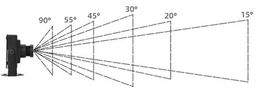
The field of view (FOV) determines how much of the scene your camera can see — essentially, how "zoomed in" or "zoomed out" your view is. In our camera class, we specify the vertical field of view in degrees:

A vertical FOV of 20 degrees creates a fairly narrow view, similar to a telephoto lens. Objects appear larger and closer. If you increased this to 90 degrees, you'd get a wide-angle view where objects appear smaller and more of the scene fits in the frame.

To use the FOV in our calculations, we first convert it to radians and then compute the viewport height:

The math here comes from basic trigonometry. Imagine a right triangle where the camera is at one vertex, the center of the viewport is at another, and half the viewport height extends to the third vertex. The angle at the camera is half of our vertical FOV. The tangent of this angle equals the opposite side (half the viewport height) divided by the adjacent side (the distance to the viewport, which we treat as 1 unit). Therefore, tan(theta/2) gives us half the viewport height, and we multiply by 2 to get the full height.

The viewport width depends on both the viewport height and the aspect ratio of our image:

The aspect ratio is the ratio of image width to image height. For example, a 400×225 image has an aspect ratio of 16:9 (approximately 1.78). By multiplying the viewport height by this ratio, we ensure that the viewport has the same proportions as our final image. This prevents distortion — circles in your scene will render as circles, not ovals.

If you set vfov = 90, you'd get a much wider view. The viewport would be taller, and more of the scene would be visible vertically. Conversely, vfov = 10 would create a very narrow, zoomed-in view where only a small portion of the scene is visible.

Now we need to position our viewport in 3D space and figure out how to map pixel coordinates to points on that viewport. The viewport sits in front of the camera, perpendicular to the viewing direction, at a distance of 1 unit (this is arbitrary — what matters is the ratio of viewport size to distance, which is determined by the FOV).

First, we express the viewport's dimensions in terms of our camera coordinate system:

The vector viewport_u spans the full width of the viewport, pointing to the right. The vector viewport_v spans the full height, but notice the negative sign — it points downward. This is because, in our image, pixel row 0 is at the top, but in our camera's coordinate system, v points upward. By negating it, we ensure that as we increment the row index, we move down the viewport.

Next, we compute how much we move for each pixel:

These vectors represent the spacing between adjacent pixels. If your image is 400 pixels wide, then pixel_delta_u is 1/400th of the viewport width. Moving from pixel column 0 to column 1 means moving by pixel_delta_u in 3D space.

Now we need to find the location of the upper-left corner of the viewport:

Starting from the camera center, we move forward by 1 unit (subtracting w because w points backward), then move left by half the viewport width and up by half the viewport height. Remember that viewport_v is already negative, so subtracting it actually moves us up.

With all the setup complete, generating a ray for a specific pixel becomes straightforward. The get_ray() function takes pixel coordinates (i, j) and returns a ray:

We start by adding jitter to the pixel coordinates. Instead of always shooting a ray through the exact center of pixel (i, j), we add a random offset between -0.5 and +0.5 in both directions. This means our sample point can be anywhere within the pixel's area. This jittering is crucial for anti-aliasing — by taking multiple samples per pixel with different jitter values, we smooth out jagged edges in the final image.

Next, we compute the 3D location of this sample point. We start at pixel00_loc (the center of the first pixel), then move right by i + jitter.x() pixel widths and down by j + jitter.y() pixel heights. This gives us a point on the viewport in 3D space.

Finally, we create a ray that starts at the camera center and points toward this sample point. The ray's direction is pixel_sample - center, which is the vector from the camera to the point on the viewport. This ray will travel through the scene, potentially hitting objects and bouncing around according to the materials it encounters.

When you call cam.render(world), the camera loops through every pixel, calling multiple times per pixel (controlled by ). Each ray traces through the scene, accumulates color from materials and lighting, and contributes to the final pixel color. The jittering ensures that each sample is slightly different, producing a smoother, more realistic image.

In this lesson, you've learned how a camera transforms high-level positioning parameters into the rays that render your scene. The camera uses lookfrom, lookat, and vup to establish its position and orientation in 3D space. From these, it constructs an orthonormal basis (u, v, w) that defines its own coordinate system.

The field of view determines how much of the scene is visible, affecting the viewport's dimensions through trigonometry. The aspect ratio ensures that the viewport matches your image proportions, preventing distortion. The camera then maps this viewport into 3D space, computing the location of each pixel and generating rays that pass through them.

The get_ray() function brings it all together, adding jitter for anti-aliasing and creating rays that originate at the camera and pass through sample points on the viewport. These rays then trace through your scene, bouncing off materials and accumulating color to produce the final rendered image.

In the upcoming practice exercises, you'll experiment with different camera parameters. You'll move the camera to different positions, point it at various targets, adjust the field of view to see how it affects the "zoom" level, and observe how these changes impact your rendered images. This hands-on experience will solidify your understanding of camera geometry and give you the skills to position your camera for compelling shots of any scene you create.