Classifying Unfamiliar Variables
Introduction
Welcome back to Which Distribution Is It? You have reached the third and final lesson of this course — and the last stop on the entire learning path. That is a big milestone! In the first lesson, we built a set of diagnostic questions for narrowing a variable to its likely distribution family. In the second lesson, we learned how to tell apart families that look similar by zeroing in on their deciding features. Now it is time to combine everything into a single, smooth reasoning process. In this lesson, you will practice classifying unfamiliar real-world variables from start to finish and learn how to justify each choice with clear evidence. We will also address an important reality: real data is never a perfect textbook shape, so every classification is an approximation, not an exact label.
From Diagnosis to Justification
So far, you have gathered two powerful skill sets. The diagnostic questions from Lesson 1 help you narrow down which family a variable likely belongs to. The distinguishing features from Lesson 2 help you confirm your choice when two families look alike. What remains is putting those skills together into a complete argument that someone else could read and find convincing.
Think of it like a doctor's visit. Asking screening questions is the first step, but the doctor also needs to explain why they reached a particular diagnosis, pointing to specific evidence. Our goal in this lesson is the same: not just picking a distribution family, but stating the reasoning clearly enough that it stands on its own.
A Three-Step Classification Workflow
When you encounter an unfamiliar variable and need to decide which distribution family fits best, the following three steps provide a reliable path from first impression to justified conclusion.
- Identify the process. Ask how the data is generated. Is every outcome equally likely? Is it a count of successes in a fixed number of yes/no trials? Is it shaped by many small, independent influences adding together? Is there a natural floor or ceiling that allows extreme values on one side?
- Check the shape. Consider what the distribution would look like. Is it flat, bell-shaped, or lopsided? If bell-shaped, is it symmetric or does one tail stretch further? Are the values whole numbers with a fixed upper limit, or continuous with no firm boundary?
- State and justify. Name the distribution family and give two pieces of evidence: one from the process (Step 1) and one from the expected shape (Step 2). This two-pronged justification is what turns a guess into a well-supported classification.
This workflow can also be pictured as a quick decision path:
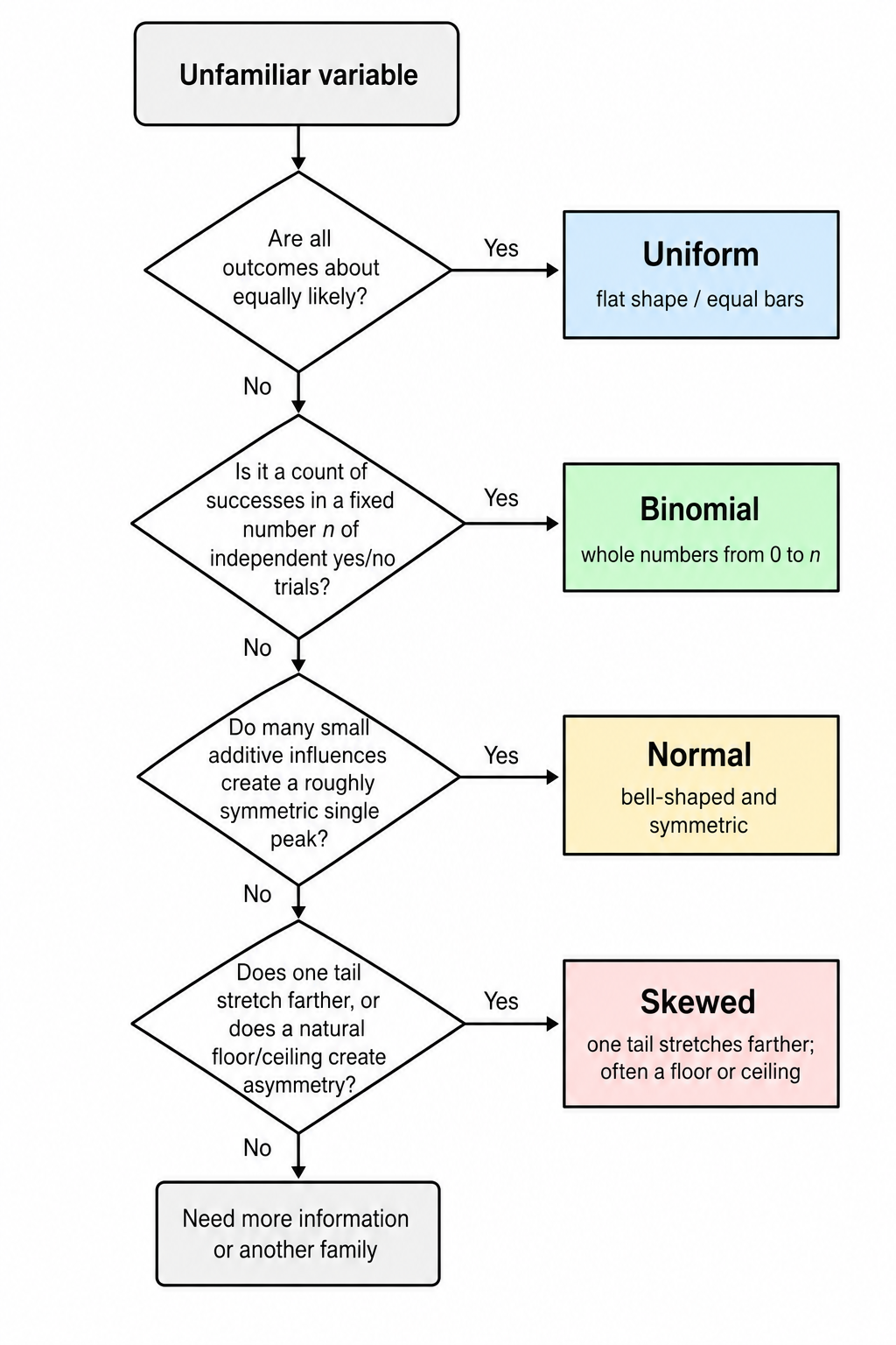
These steps are not new ideas — they simply organize the diagnostic questions and distinguishing features you already know into a repeatable workflow.
Worked Examples: Classifying Unfamiliar Variables
Let us walk through four quick examples, one for each family, to see the workflow in action. The visual below summarizes the expected shapes behind the four examples.
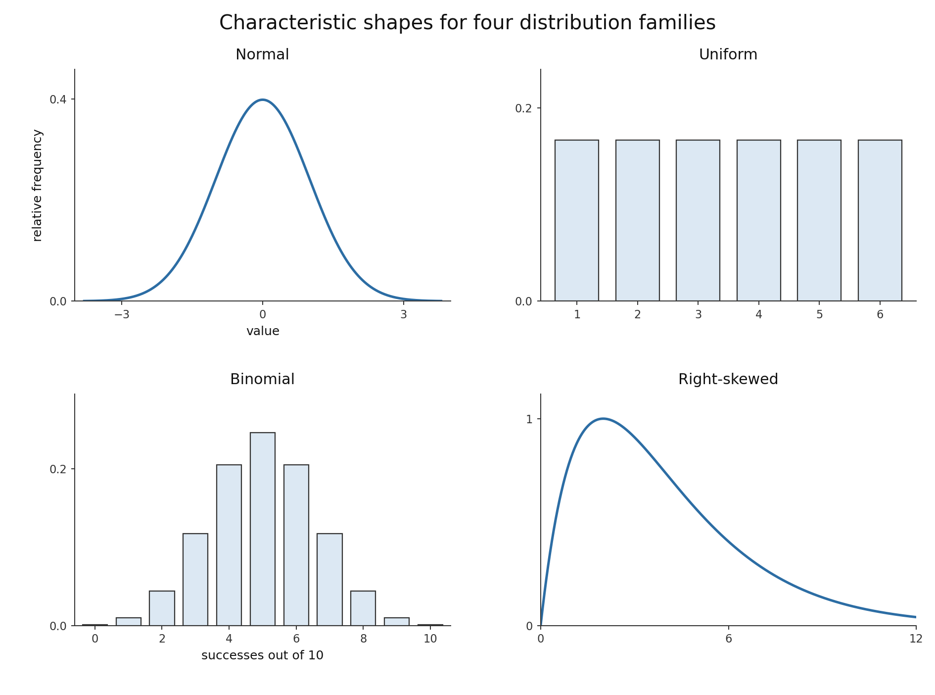
Example 1 — Heights of adult women in a large city. The process: a person's height results from genetics, nutrition, and many other small, independent factors that combine additively. The shape: we expect a single peak at the most common height, with values tapering symmetrically on both sides. Classification: normal. The many-small-influences process and the symmetric bell shape both point to the normal family.
Example 2 — The number shown on a fair six-sided die. The process: each face has an equal chance, and no outcome is favored. The shape: a flat bar chart with six bars of equal height. Classification: uniform. Equal likelihood across all outcomes is the hallmark of the uniform distribution.
Example 3 — Free throws made out of attempts by a basketball player. The process: there are independent yes/no trials (made or missed), each with roughly the same success probability. The variable is a whole-number count ranging from to . Classification: binomial. The fixed number of independent yes/no trials and the integer-valued outcome fit the binomial setup exactly.
Example 4 — Sale prices of homes in a mid-sized city. The process: most homes cluster around a moderate price, but there is a hard floor near zero (prices cannot be negative) and no firm ceiling, allowing a handful of luxury properties to stretch far to the right. The shape: a single peak with a long right tail. Classification: right-skewed. The floor-plus-no-ceiling mechanism and the asymmetric tail are signatures of right skew.
Notice that every classification above includes both a process reason and a shape reason. That two-part structure is what makes a justification convincing.
Real Data Only Approximates Named Shapes
Up to now, we have talked about distributions as if real data falls neatly into one of our four families. In practice, it rarely does.
Real-world data is influenced by measurement quirks, sample size limits, mixed subgroups, and countless other irregularities. A histogram of actual adult heights might have a small bump on one side. Actual home prices might show a second minor peak near a popular price point. These imperfections do not mean our classification is wrong — they mean the named shape is a useful model, not an exact description.
When justifying a classification, it is good practice to acknowledge this gap between model and reality. A simple qualifier does the job:
- "The distribution is approximately normal because…"
- "This variable is roughly right-skewed, though real data may show minor irregularities."
The word approximately signals that you understand the difference between an idealized model and messy reality. It also protects your reasoning: if someone points out a small deviation in the data, your conclusion still holds because you never claimed a perfect fit.
Writing a Complete Justification
Let us put all the pieces together into a short template you can follow whenever you need to classify and justify a variable:
- Name the variable and briefly describe what it measures.
- State the distribution family using a qualifier like approximately or most likely.
- Give process evidence explaining how the data is generated and why that mechanism matches the chosen family.
- Give shape evidence describing the expected visual features (symmetry, peaks, tails, value type).
- Acknowledge approximation by noting that real data may not match the ideal shape perfectly.
Here is a sample justification that follows this template:
Monthly electricity bills for households in a city are most likely right-skewed. Most households use a moderate amount of electricity, so bills cluster around a typical value, with a natural floor near zero since a bill cannot be negative. However, homes with heavy air conditioning, pools, or high-demand equipment can run up much larger bills, stretching the right tail well beyond the peak. We would expect a single peak in the low-to-moderate range with a long tail to the right. In practice, the histogram may show secondary bumps — for example, around common rate-plan thresholds — so the skewed shape is an approximation rather than a perfect fit.
This justification hits every element: it names the variable, states the family with a qualifier, provides process and shape evidence, and acknowledges that real data is only an approximation.
Conclusion and Next Steps
In this lesson, you combined the diagnostic questions and distinguishing features from the first two lessons into a single three-step workflow: identify the process, check the shape, and state your justified conclusion. You practiced classifying variables across all four families and learned that a strong justification always includes both process evidence and shape evidence, along with an honest acknowledgment that real data only approximates ideal named shapes.
You now have everything you need to classify unfamiliar variables with confidence. Head into the practice exercises to put this skill to work — you will pick distribution families for new variables, match real-world scenarios to their correct distributions, complete a structured justification, and write one entirely on your own. Time to show what you have learned across this entire path!
