Welcome back to Vertical Shifts: Moving Graphs Up and Down. This is the third and final lesson of the course, and it is where we run the machinery backwards. Until now, someone handed us an equation and we produced a picture. From here on, someone hands us a picture and we produce the equation.
That reversal matters because real data rarely arrives as a formula. A parking meter's price chart, a payroll graph, a bank balance plotted over time—these show up as lines and curves on a screen, and the useful question is always the same: what constant was added to get them there? By the end of this lesson, we will be able to measure k off a graph, write f(x)+k with the correct sign, choose the k that lands on a target y-intercept, and say precisely what that constant did and did not change.
The Anchor Is the Fingerprint
Each parent graph from the first lesson carries an anchor point that sits at the origin: the vertex of y=x2, the corner of y=∣x∣, the endpoint of y=x, and the origin crossing of y=x. Those anchors are the most recognizable spots on each curve, which is exactly why they are so useful in reverse.
Because a vertical shift is rigid, the anchor travels with the graph and lands exactly k units from where it started. Nothing else about the picture changes, so all the information about the shift is concentrated in that one point. Spot a familiar shape resting at an unfamiliar height, and the anchor tells the whole story at a glance.
Measuring the Displacement
The routine is short: identify the parent shape, locate its anchor on the shifted graph, and compare that height to the original anchor height.
k=ynew−yold
Since all four of our parent anchors start at y=0, this simplifies beautifully—the height of the anchor is k. A V-shaped graph whose corner sits at (0,−4) has k=−4. A square-root curve beginning at (0,2) has k=2.
For example, compare the parent V’s corner at (0,0) with a shifted V’s corner at (0,−4). The unchanged V shape confirms that the transformation is rigid, and the four-unit downward displacement gives k=−4.
The subtraction order is worth locking in, because reversing it flips every sign you produce. New minus old, always: above the original means positive, below means negative, and the magnitude is simply the vertical gap you counted.
Join the 1M+ learners on CodeSignal
Be a part of our community of 1M+ users who develop and demonstrate their skills on CodeSignal
Once k is measured, the equation writes itself. Take the parent formula and attach the constant with its own sign—we never write a plus in front of a negative k, we fold the sign in and read it directly.
What the graph shows
Measured k
Equation
Parabola with vertex (0,5)
+5
y=x2+5
V with corner (0,−4)
−4
y=∣x∣−4
Square-root curve starting at (0,2)
+2
y=x+2
Straight line through (0,−1) at 45∘
−1
y=x−1
Two graphs can shift in the same direction and still be different functions, so the size of k deserves as much attention as its sign. A parabola resting at (0,1) and one resting at (0,6) are both shifted up, but only one of them is y=x2+6.
An anchor can be misread, especially on a coarse grid, so a few seconds of checking pays off. Pick any convenient x, compute what the parent would give there, and compare it to the height you actually see. The difference must equal the k you already measured.
Suppose we read a parabola's vertex as (0,−3) and want to be sure. At x=2 the parent gives 22=4, so the shifted curve should pass through (2,4−3)=(2,1). If the graph really does sit at height 1 above x=2, our k is confirmed.
This trick also rescues us when the anchor is off-screen entirely. Any single visible point is enough, since k=ygraph−f(x) holds at every input, not just at the anchor.
Now let us turn the problem into a design decision: instead of reporting the shift we see, we choose the shift we want. The y-intercept of a shifted function is the original intercept plus the constant,
g(0)=f(0)+k
so aiming at a specific crossing height means solving k=target−f(0). For a parent graph, f(0)=0 and the answer is immediate: to make y=x+k meet the axis at 7, take k=7.
The interesting case is when the original function does not pass through the origin. If f(0)=3 and we need the shifted graph to cross at −2, then k=−2−3=−5, giving g(x)=f(x)−5. That is precisely the arithmetic a pricing analyst runs when a total has to start at a particular number.
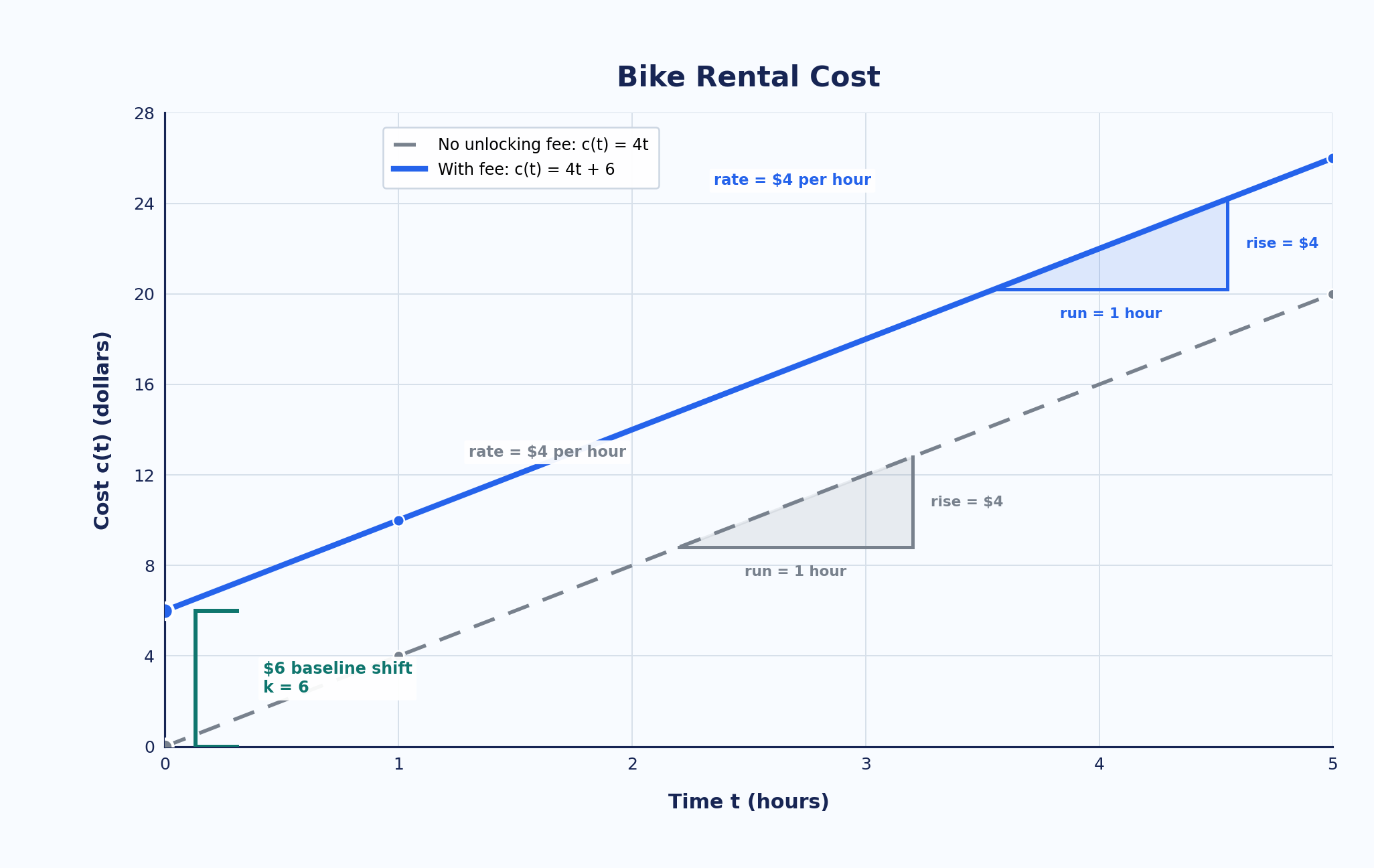
In applied settings, k almost always means a baseline: a starting amount, a flat fee, an opening balance. Think of a bike rental that charges $4 per hour. Without a fee the cost is c(t)=4t; add a $6 unlocking charge and it becomes c(t)=4t+6, a graph lifted six units with k=6.
The two parallel cost lines below show the starting amount changing while the hourly rate holds steady.
The part that is easy to overstate is what actually changed. Every total moved up by $6, but the per-hour rate is untouched: two hours still cost $8 more than zero hours, exactly as before. A lowered starting balance behaves the same way with k negative—every total drops, while the rate of change carries on unaffected.
Reverse-engineering has its own small set of traps, and each one is quick to defuse.
Mix-up
How to settle it
Counting the gap horizontally
A vertical shift only moves heights. Compare the two anchors along a vertical line, never a diagonal or sideways one.
Computing yold−ynew
The sign comes out backwards every time. Fix the order as new minus old and stick to it.
Assuming the y-intercept is always k
That holds only when f(0)=0, which is true for our four parents but not in general. Otherwise use k=target−f(0).
If a reading ever feels shaky, fall back on the second-point check from earlier. One extra coordinate settles almost every dispute about sign or size.
We can now read a graph and recover the constant behind it. Measure the anchor's displacement as new minus old, attach that signed k to the parent formula, confirm it with one extra point, and solve k=target−f(0) whenever a specific intercept is required. Just as importantly, we can explain the result in plain language: the baseline moved, while the shape, the steepness, and the allowed inputs stayed exactly as they were.
The practice ahead is where this becomes second nature. You will measure signed shifts from rendered graphs, match plotted curves to equations that differ in both sign and size, tune a constant until it hits a chosen intercept, and sort baselines from rates in salary and balance scenarios. The finale is a real parking-cost graph, where you will write the equation, verify it against the intercept, and explain what the entry charge leaves alone.