ReLU Activation and Flexible Layer Design in R MLPs
Introduction
Welcome to the second lesson of our course on the MLP architecture: activations & initialization! We're making excellent progress on our neural network journey. In the previous lesson, we successfully implemented a multi-layer perceptron (MLP) by stacking multiple dense layers, allowing information to flow from input to output through our network.
Today, we'll be exploring an essential component of modern neural networks: the rectified linear unit (ReLU) activation function. While we've been using the sigmoid activation function so far, ReLU has become the default activation function for most hidden layers in deep neural networks due to its computational efficiency and effectiveness in addressing the vanishing gradient problem.
By the end of this lesson, you'll understand what ReLU is, why it's so popular, and how to implement and incorporate it into your neural network architecture. We'll also modify our DenseLayer class to support different activation functions, making our neural network framework more flexible and powerful. Let's dive in!
Understanding Activation Functions and Their Importance
As we've seen in our previous work, activation functions introduce non-linearity into our neural networks. Without them, no matter how many layers we stack, our network would merely compute a linear transformation of the input data.
Let's quickly recall the sigmoid activation function we've been using:
The sigmoid function maps any input to a value between 0 and 1, creating a smooth S-shaped curve. While it works well for certain tasks, sigmoid has some significant limitations:
Vanishing Gradients: When inputs are very large or very small, the gradient of the sigmoid function becomes extremely small, slowing down learning. We'll be discussing gradients in much more detail in our next course about training neural networks, but for the time being, you can think of the gradient as the fundamental feedback signal that the network uses to adapt its weights and learn.
Computational Expense: Computing exponentials is relatively expensive.
Not Zero-Centered: The output is always positive, which can cause zig-zagging dynamics during optimization.
These limitations become particularly problematic in deep networks with many layers. This is where alternative activation functions like ReLU come into play, offering solutions to many of these challenges.
Join the 1M+ learners on CodeSignal
Be a part of our community of 1M+ users who develop and demonstrate their skills on CodeSignal
The ReLU Activation Function
Implementing the ReLU Activation Function
Let's implement the ReLU activation function in R. The implementation is remarkably simple:
relu <- function(x) { return(pmax(x, 0))}
This leverages R's pmax function, which returns the element-wise maximum between two values. In this case, we're comparing each element of x with 0 and taking the larger value. The beauty of using R's vectorized operations is that this will work efficiently whether x is a single value, a vector, or a matrix, and pmax automatically preserves the dimensions of the input.
When we apply ReLU to matrices of weighted sums in our neural network, all positive values will remain unchanged, while all negative values will be replaced with zeros.
Modifying Our DenseLayer for Different Activations
Building an MLP with Mixed Activations
Examining ReLU Behavior with Different Inputs
Conclusion and Next Steps
Great work! You've now learned about the ReLU activation function, its advantages over sigmoid, and how to implement and use it in your neural network framework using R6 classes. You've also seen how to build MLPs with mixed activation functions and observed the unique behavior of ReLU in practice.
Up next, you'll get hands-on experience with a practice section focused on ReLU, where you'll solidify your understanding by applying what you've learned. After that, we'll move on to discuss activation functions specifically designed for output layers, such as linear and softmax activations, and see how they are used for different types of prediction tasks. Your neural network toolkit is expanding, and you're well on your way to building more flexible and powerful models!
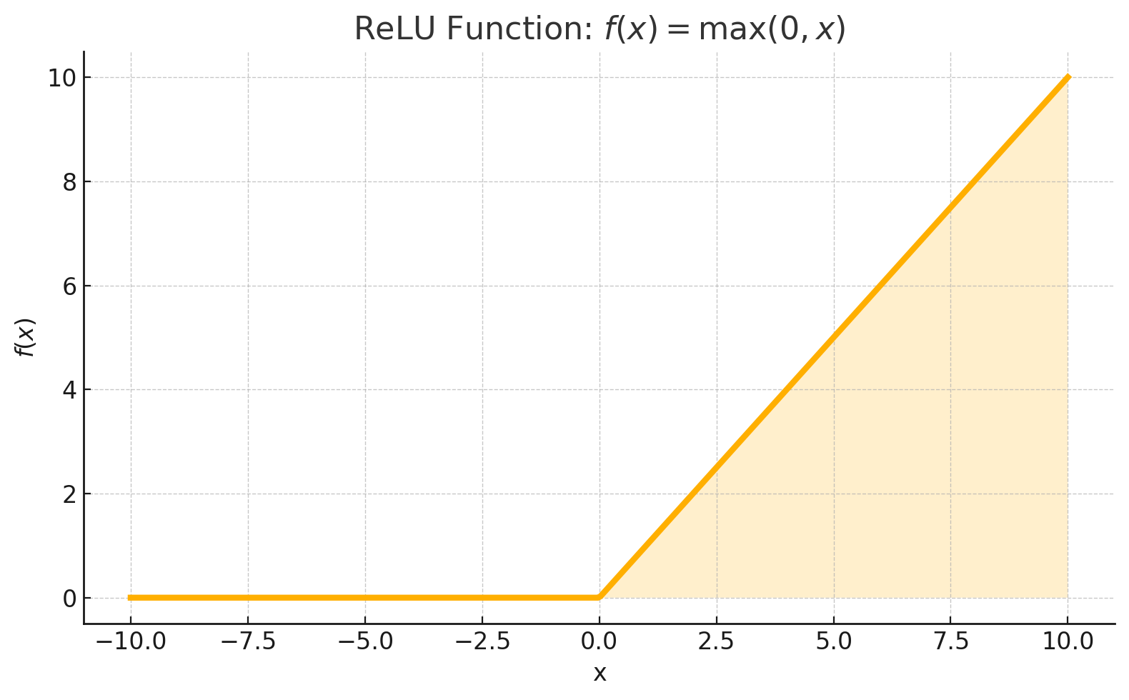
The rectified linear unit (ReLU) is perhaps the simplest non-linear activation function, yet it has revolutionized deep learning. Its mathematical definition is elegantly straightforward:
f(x)=max(x,0)
In plain English: ReLU outputs the input directly if it's positive and outputs zero if the input is negative. This creates a simple "ramp" function that's linear for positive values and flat for negative values.
The advantages of ReLU over sigmoid are numerous and significant:
Computational Efficiency: ReLU involves only a simple max operation, making it much faster to compute than functions involving exponentials.
Reduced Vanishing Gradient Problem: For positive inputs, the gradient is always 1, allowing for much faster learning.
Sparsity: ReLU naturally creates sparse activations (many neurons output zero), which can be beneficial for representation learning.
Biological Plausibility: The firing pattern of ReLU resembles that of biological neurons more closely than sigmoid.
These advantages have made ReLU the default choice for hidden layers in most modern neural networks. However, it's worth noting that ReLU also has a limitation known as the "dying ReLU problem" — neurons can get stuck in a state where they always output zero, effectively becoming "dead" and unable to learn.
R
relu <- function(x) { return(pmax(x, 0))}
Now that we have both sigmoid and ReLU activation functions, let's modify our DenseLayer class to support different activation functions. This will make our neural network architecture more flexible. We'll use R6 classes for better object-oriented programming practices:
Used the R6 class system to create a proper class definition with public fields and methods.
Added an activation_fn_name parameter to the constructor, defaulting to 'sigmoid' for backward compatibility.
Stored the activation function name as a field in the class for informational purposes.
Added logic to select the appropriate activation function based on the provided name.
Improved bias broadcasting to handle multiple input samples properly.
Added error handling for unsupported activation functions.
This approach offers several benefits:
It provides better object-oriented programming practices with proper encapsulation.
It maintains backward compatibility with our existing code.
It makes our layer's behavior more transparent (we can easily see which activation is being used).
It sets us up to add more activation functions in the future.
With our enhanced DenseLayer class, we can now create an MLP that uses different activation functions for different layers. This is a common practice in deep learning, where ReLU is typically used for hidden layers and sigmoid (or softmax) for the output layer, depending on the task.
Let's build an MLP with ReLU for the first layer and sigmoid for the subsequent layers:
R
# Create sample inputsX_sample <- matrix(c(-1.0, 0.5, 2.0, -0.1, 1.0, 0.5, 2.0, 0.1), nrow = 2, ncol = 4, byrow = TRUE)cat("Input X (shape", paste(dim(X_sample), collapse = " x "), "):\n")print(X_sample)# Create the MLP with mixed activationsmlp_relu <- MLP$new()mlp_relu$add_layer(DenseLayer$new(n_inputs = 4, n_neurons = 5, activation_fn_name = 'relu'))mlp_relu$add_layer(DenseLayer$new(n_inputs = 5, n_neurons = 3, activation_fn_name = 'sigmoid'))mlp_relu$add_layer(DenseLayer$new(n_inputs = 3, n_neurons = 1, activation_fn_name = 'sigmoid'))# Display information about our network architecturecat("\nMLP created with", length(mlp_relu$layers), "layers and mixed activations.\n")for (i in seq_along(mlp_relu$layers)) { layer <- mlp_relu$layers[[i]] cat(" Layer", i, ":", layer$n_inputs, "inputs,", layer$n_neurons, "neurons, Activation:", layer$activation_fn_name, "\n")}
This creates a 3-layer MLP with:
A first layer using ReLU activation with 5 neurons.
A second layer using sigmoid activation with 3 neurons.
An output layer using sigmoid activation with 1 neuron.
Let's see what happens when we forward propagate our input through this network with mixed activations:
R
# Forward passoutput_relu <- mlp_relu$forward(X_sample)cat("\nOutput of the MLP (shape", paste(dim(output_relu), collapse = " x "), "):\n")print(output_relu)
This gives us something like:
Output of the MLP (shape 2 x 1): [,1][1,] 0.5210851[2,] 0.5215234
Our MLP with mixed activations is working! But to really understand how ReLU affects our network, let's try an input with mostly negative values:
# Test with mostly negative valuesX_negative_heavy <- matrix(c(-1.0, -0.5, -2.0, -0.1, -2.0, -0.1, -3.0, -1.1), nrow = 2, ncol = 4, byrow = TRUE)cat("\nInput with mostly negative values (shape", paste(dim(X_negative_heavy), collapse = " x "), "):\n")print(X_negative_heavy)# Forward propagate and examine the first layer's outputoutput_negative_heavy <- mlp_relu$forward(X_negative_heavy)cat("Output for negative heavy input (shape", paste(dim(output_negative_heavy), collapse = " x "), "):\n")print(output_negative_heavy)cat("Output of first layer (ReLU) after forward pass:\n")print(mlp_relu$layers[[1]]$output)
The result reveals a fascinating aspect of ReLU:
Input with mostly negative values (shape 2 x 4): [,1] [,2] [,3] [,4][1,] -1 -0.5 -2 -0.1[2,] -2 -0.1 -3 -1.1Output for negative heavy input (shape 2 x 1): [,1][1,] 0.5209758[2,] 0.5209234Output of first layer (ReLU) after forward pass: [,1] [,2] [,3] [,4] [,5][1,] 0 0 0 0 0[2,] 0 0 0 0 0
Look at the output of the first layer! It's all zeros for both input samples. This illustrates a key property of ReLU: it completely blocks negative inputs, resulting in a sparse activation pattern. In this case, all of our input values resulted in negative weighted sums in the first layer, so ReLU converted them all to zeros.
Despite this extreme first-layer output, our network still produced a non-zero final output. Here's why: even though the first layer outputs all zeros and biases are initialized to zero, when these zeros are passed to the second layer, the weighted sum becomes zero: 0 × weights + 0 = 0. However, the sigmoid activation function transforms this: sigmoid(0) = 0.5. So each neuron in the second layer outputs approximately 0.5, allowing information to continue flowing through the network.
This example highlights the importance of proper weight initialization and careful network design when using ReLU. If too many neurons "die" (always output zero), the network's capacity to learn can be severely limited.
R
# Test with mostly negative valuesX_negative_heavy <- matrix(c(-1.0, -0.5, -2.0, -0.1, -2.0, -0.1, -3.0, -1.1), nrow = 2, ncol = 4, byrow = TRUE)cat("\nInput with mostly negative values (shape", paste(dim(X_negative_heavy), collapse = " x "), "):\n")print(X_negative_heavy)# Forward propagate and examine the first layer's outputoutput_negative_heavy <- mlp_relu$forward(X_negative_heavy)cat("Output for negative heavy input (shape", paste(dim(output_negative_heavy), collapse = " x "), "):\n")print(output_negative_heavy)cat("Output of first layer (ReLU) after forward pass:\n")print(mlp_relu$layers[[1]]$output)