Welcome to The Correlation Coefficient, the second course in this learning path! In the previous course, Seeing Relationships in Data, we learned how to spot patterns in scatter plots and describe them using three qualities: direction, strength, and form. Now we take the next step and turn that visual impression into a single number.
This first lesson focuses on interpreting the correlation coefficient. By the end, you will know exactly what this number can (and cannot) tell you, how to read its sign, how to judge its magnitude, and what happens at three benchmark values. Let's get started.
From Visual Impressions to a Precise Number
As you may recall from the previous course, we described relationships as "strong positive" or "weak negative" just by looking at scatter plots. That approach works, but it is subjective — two people can look at the same cloud of points and disagree on whether it is "moderate" or "strong."
The correlation coefficient, denoted by r, solves this problem by assigning a single numerical value to the strength and direction of a linear relationship between two quantitative variables. Instead of debating words, we can point to a number and have a shared, precise language. Think of it like replacing "it feels warm outside" with "it is 78 °F" — the number removes ambiguity.
The Range of r
The correlation coefficient always falls between −1 and +1, inclusive. We can write this compactly as:
−1≤r≤+1
No matter what data set you work with, r will never drop below −1 or rise above +1. This fixed scale is what makes the coefficient so convenient: once you know this range, every value you encounter is immediately comparable to every other.
When r is Undefined: While r usually falls between −1 and +1, it cannot be calculated in two specific cases:
If you have fewer than two pairs of data.
If all the values for one variable are the same (e.g., if everyone in a study is exactly the same height). In this case, the standard deviation is zero, and the formula fails.
With the range established, the next question is what each part of r — its sign and its size — actually tells us.
What the Sign Tells Us: Direction
Join the 1M+ learners on CodeSignal
Be a part of our community of 1M+ users who develop and demonstrate their skills on CodeSignal
The sign of r (positive or negative) tells us the direction of the linear association:
Positive r: As one variable increases, the other tends to increase as well. Think of height and shoe size — taller people generally wear larger shoes.
Negative r: As one variable increases, the other tends to decrease. Think of outdoor temperature and home heating cost — warmer weather usually means lower bills.
r equal to zero: There is no consistent upward or downward linear trend, so the sign carries no directional meaning.
The sign alone, however, does not tell us how closely the data follow the trend. For that, we need to look at the size of r.
The magnitude (absolute value) of r, written ∣r∣, tells us how tightly the points cluster around a straight line. The closer ∣r∣ is to 1, the stronger the linear pattern; the closer it is to 0, the weaker.
While thresholds can vary by field, the following inequalities provide a standard convention for classifying strength:
Magnitude Range
Informal label
0.0<∣r∣<0.3
Weak
0.3≤∣r∣<0.7
Moderate
0.7≤∣r∣<1.0
Strong
These labels are guidelines, not strict laws. A helpful analogy is a volume knob — turning from 0 toward 1 makes the linear signal louder and clearer. Using inequalities ensures that every possible value, like 0.295 or 0.699, has a clear classification.
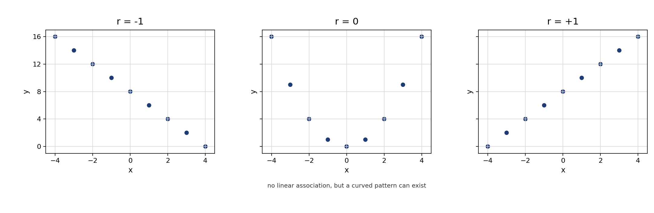
Three specific values deserve extra attention. While −1 and +1 are the boundaries of the possible range, 0 represents the midpoint. Together, these serve as benchmarks for the extreme cases of what r can describe.
r=+1: Every data point falls exactly on a line that slopes upward. The linear relationship is perfect and positive.
r=−1: Every data point falls exactly on a line that slopes downward. The linear relationship is perfect and negative.
r=0: There is no linear association between the variables. This does not mean the variables are unrelated in every possible way — it only means that a straight line does a poor job summarizing their pattern. A perfect curve, for example, could still be hiding in the data.
Understanding r=0 is especially important. A common misconception is that r=0 means "no relationship at all." In reality, it only rules out a linear one.
Notice that the middle plot shows a clear curved pattern even though r=0. The coefficient only measures how well a straight line fits the data, so a strong non-linear pattern can exist right under its nose.
Interpreting r always involves two quick steps: check the sign to determine direction (positive or negative), then check the magnitude to judge strength (weak, moderate, or strong).
For example, suppose a researcher reports that the correlation between daily study time and exam score is r=0.72. The positive sign tells us that more study time is associated with higher scores. The magnitude of 0.72 falls in the "strong" range (0.7≤∣r∣<1.0), so the points cluster fairly closely around an upward-sloping line. In one short sentence we might say: "There is a strong, positive linear association between daily study time and exam score."
Now consider r=−0.22 for the relationship between commute distance and job satisfaction. The negative sign means longer commutes tend to go with lower satisfaction. The magnitude of 0.22 sits in the "weak" range (0.0<∣r∣<0.3), so the trend exists but the points are widely scattered. We would describe this as a weak, negative linear association.
In this lesson we established the four foundational facts about the correlation coefficient r: it ranges from −1 to +1, its sign indicates direction, its magnitude indicates strength, and the benchmark values −1, 0, and +1 each tell a clear story about how data points relate to a straight line. Keep in mind that r=0 means no linear association, not necessarily no relationship at all. These ideas form the backbone of everything else we will explore in this course.
Up next, you will put these concepts into action with a set of hands-on practice tasks. You will fill in key facts about r, match coefficient values to verbal descriptions, interpret benchmark cases, and write your own real-world interpretation!