Aggregating Order Value by Customer

Welcome back to Structuring Queries with Common Table Expressions. We have completed the first two lessons, and we are now at Lesson 3 in Unit 3 of 4. Previously, we connected order-total calculations and customer details in a chained pipeline. Today, we will change the report’s level of detail: first, keep one prepared total per order; then, combine those totals into one summary per customer; and finally, add readable names.

We will focus on how each CTE passes a clear row shape to the next stage. By the end, we will have a customer order value report with order counts, rounded order value, and deterministic ordering.

order_totals is the same stage established in Lesson 2, unchanged here. Its contract is one row per order_id, each carrying a rounded order_total. That contract establishes the starting grain—one row per order—for the customer-level aggregation that follows.

WITH order_totals AS (
    SELECT
        oi.order_id,
        ROUND(SUM(oi.quantity * p.product_price), 2) AS order_total
    FROM OrderItems AS oi
    INNER JOIN Products AS p
        ON p.product_id = oi.product_id
    GROUP BY oi.order_id
),

The stage's narrow contract is the important part here: later stages can consume a prepared order total without returning to the item rows. The calculation itself remains isolated in this CTE.

The next stage connects each prepared total to the order record that owns it. Orders provides customer_id, while the earlier CTE provides order_total. Since order_totals contains one row per order_id and Orders contains one row per order, this join keeps the order level of detail instead of aggregating too early.

customer_orders AS (
    SELECT
        o.customer_id,
        ot.order_total
    FROM Orders AS o
    INNER JOIN order_totals AS ot
        ON ot.order_id = o.order_id
),

The stage projects only what the next aggregation needs: the customer_id that defines the group and the prepared order_total that will be summed. Keeping the projection narrow makes the stage's contract obvious—one row per order, attributed to a customer. The comma after this CTE separates it from the next stage in the complete WITH clause.

Now we can change the row grain deliberately. customer_orders has one row per order, so grouping by customer_id creates one row per customer. This is the right moment to count orders and add order value because each source row represents exactly one order and already contains its calculated total.

customer_totals AS (
    SELECT
        customer_id,
        COUNT(*) AS order_count,
        ROUND(SUM(order_total), 2) AS customer_order_value
    FROM customer_orders
    GROUP BY customer_id
)

COUNT(*) counts orders, not order items, because the input has one row per order. Even though order_id is not projected, each source row still represents exactly one order. SUM(order_total) adds the prepared order values, and ROUND(..., 2) keeps customer order value consistent with the report format. Notice that we do not multiply quantities by prices again. The pipeline reuses the earlier calculation, which keeps the logic consistent and makes each stage easier to verify. This CTE now exposes customer_id, order_count, and customer_order_value.

The final query should read from customer_totals, not from the raw tables. The totals CTE already contains the measures, while Customers supplies the readable name. We join on customer_id and select only the fields needed by the report.

SELECT
    c.customer_id,
    c.customer_name,
    ct.order_count,
    ct.customer_order_value
FROM customer_totals AS ct
INNER JOIN Customers AS c
    ON c.customer_id = ct.customer_id
ORDER BY ct.customer_order_value DESC, c.customer_id

The first sort key places the highest order value first. The second sort key, c.customer_id, is unique and ascending, so it resolves equal order-value amounts and creates a total deterministic order. The result contains the customer ID, customer name, order count, and order value. Every order contributes, whatever its status, so customer_order_value measures gross order value rather than recognized revenue. We also leave the staged totals intact without repeating the item-level calculation.

We have now examined each stage in isolation. When combined, the statement follows a controlled change in grain: detailed items become orders, orders become customers, and customer summaries become a readable report. The following diagram highlights where the row grain changes and where it remains stable.

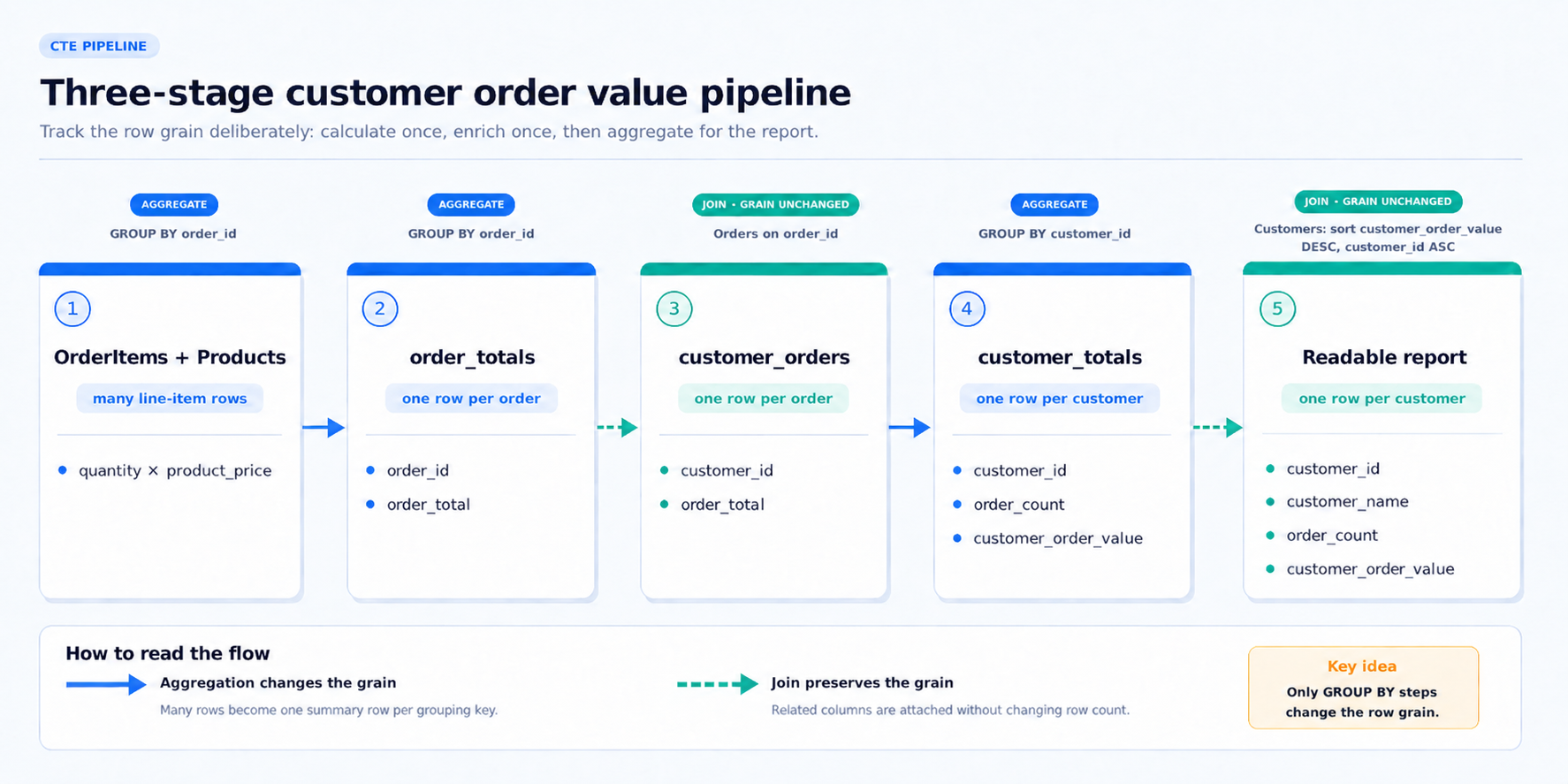
Here is the complete MySQL 8.0 statement, with each dependency declared before it is used.

WITH order_totals AS (
    SELECT
        oi.order_id,
        ROUND(SUM(oi.quantity * p.product_price), 2) AS order_total
    FROM OrderItems AS oi
    INNER JOIN Products AS p
        ON p.product_id = oi.product_id
    GROUP BY oi.order_id
),
customer_orders AS (
    SELECT
        o.customer_id,
        ot.order_total
    FROM Orders AS o
    INNER JOIN order_totals AS ot
        ON ot.order_id = o.order_id
),
customer_totals AS (
    SELECT
        customer_id,
        COUNT(*) AS order_count,
        ROUND(SUM(order_total), 2) AS customer_order_value
    FROM customer_orders
    GROUP BY customer_id
)
SELECT
    c.customer_id,
    c.customer_name,
    ct.order_count,
    ct.customer_order_value
FROM customer_totals AS ct
INNER JOIN Customers AS c
    ON c.customer_id = ct.customer_id
ORDER BY ct.customer_order_value DESC, c.customer_id;

order_totals performs the calculation, customer_orders performs the enrichment, customer_totals performs the customer aggregation, and the final SELECT performs the presentation. To make the flow concrete, imagine an order with 2 units priced at 12.50 and 1 unit priced at 30.00: its total is 55.00. If that order belongs to customer 7, the bridge carries customer 7 and 55.00 forward. If that customer has three orders totaling 55.00, 20.00, and 80.00, customer_totals returns an order count of 3 and order value of 155.00. The final join adds the customer’s name and places the row according to order value.

Staged aggregation gives each transformation a clear job. order_totals converts line-item values into one rounded total per order. customer_orders attaches customer information without changing that order level. customer_totals counts orders and sums prepared order values for each customer. The final join adds names and sorts the report by order value, then by customer ID, for deterministic results.

The broader pattern is to control row grain and pass named, verified results from one CTE to the next. This avoids repeated calculations, makes intermediate results easier to inspect, and leaves room for future reports or window functions.

In the upcoming practice section, we will inspect the starting report and relationships, build each CTE, and finish the readable customer order value report. Let’s turn this pipeline into working SQL and verify each stage as we go.