Welcome back to Slope Changes and Rates of Change. This is the third and final lesson of the course, and it hands the controls over to you: instead of adjusting a slope and watching a graph respond, you will be given the finished result and asked to explain what happened.
That reversal is exactly what real life asks of us. A gym raises its price, a phone carrier rewrites its plan, a spreadsheet arrives with two columns of numbers — and someone has to say whether the rate changed, the starting value changed, or both. In this lesson we will learn to answer that question from evidence, and then answer the follow-up that matters even more: how far apart will the two models be a month, a year, or a hundred miles from now?
Every Linear Model Carries Two Numbers
A linear model written as y=mx+b stores exactly two pieces of information, and each one answers a different question:
b is the starting value, the output when the input is 0. It is the same (0,b) pivot we studied in the last lesson, now wearing a job title.
m is the rate, the change in output for each one-unit increase in input.
The words wrapped around those numbers change with the story. In a phone plan, b is a monthly base fee and m is the cost per gigabyte; on a road trip, b is the miles already driven and m is the speed. The math stays put while only the labels move, which is why one diagnosis will work across every example in this lesson.
Reading the Rate and the Starting Value
Before diagnosing any change, we have to identify these two numbers correctly, and the safest method is to attach a unit to each. The rate always carries a "per" in its unit, while the starting value carries the output unit alone.
Consider a taxi that charges a $3.50 pickup fee plus $2.25 per mile:
C(d)=2.25d+3.50
Here 2.25 is measured in dollars per mile, so it is the rate, and 3.50 is measured in dollars, so it is the starting value. A quick check confirms it: C(0)=3.50, the price of a ride that goes nowhere.
Notice that the sentence mentions the fee first and the rate second, while the equation lists them in the opposite order. Word order is not a reliable clue — let the units decide.
Same Start, Different Rate: The Gap Grows
Join the 1M+ learners on CodeSignal
Be a part of our community of 1M+ users who develop and demonstrate their skills on CodeSignal
Same Rate, Different Start: The Gap Stays Put
Signatures: What the Evidence Tells Us
Because those two behaviors look nothing alike, we can diagnose a change from evidence rather than impression. Two features are enough: where each model crosses the vertical axis and the signed rate of each model, including whether it rises or falls.
What we observe
What changed
Same y-intercept, different signed rates
the rate only
Parallel lines, different y-intercepts
the starting value only
Different y-intercepts and different signed rates
both
Same intercept and same signed rate
nothing; the models are identical
Notice which observation is missing from that table: "the lines cross." Two lines with different slopes always meet somewhere, so a crossing point by itself proves nothing. Y-intercepts and signed rates are the evidence; everything else is decoration.
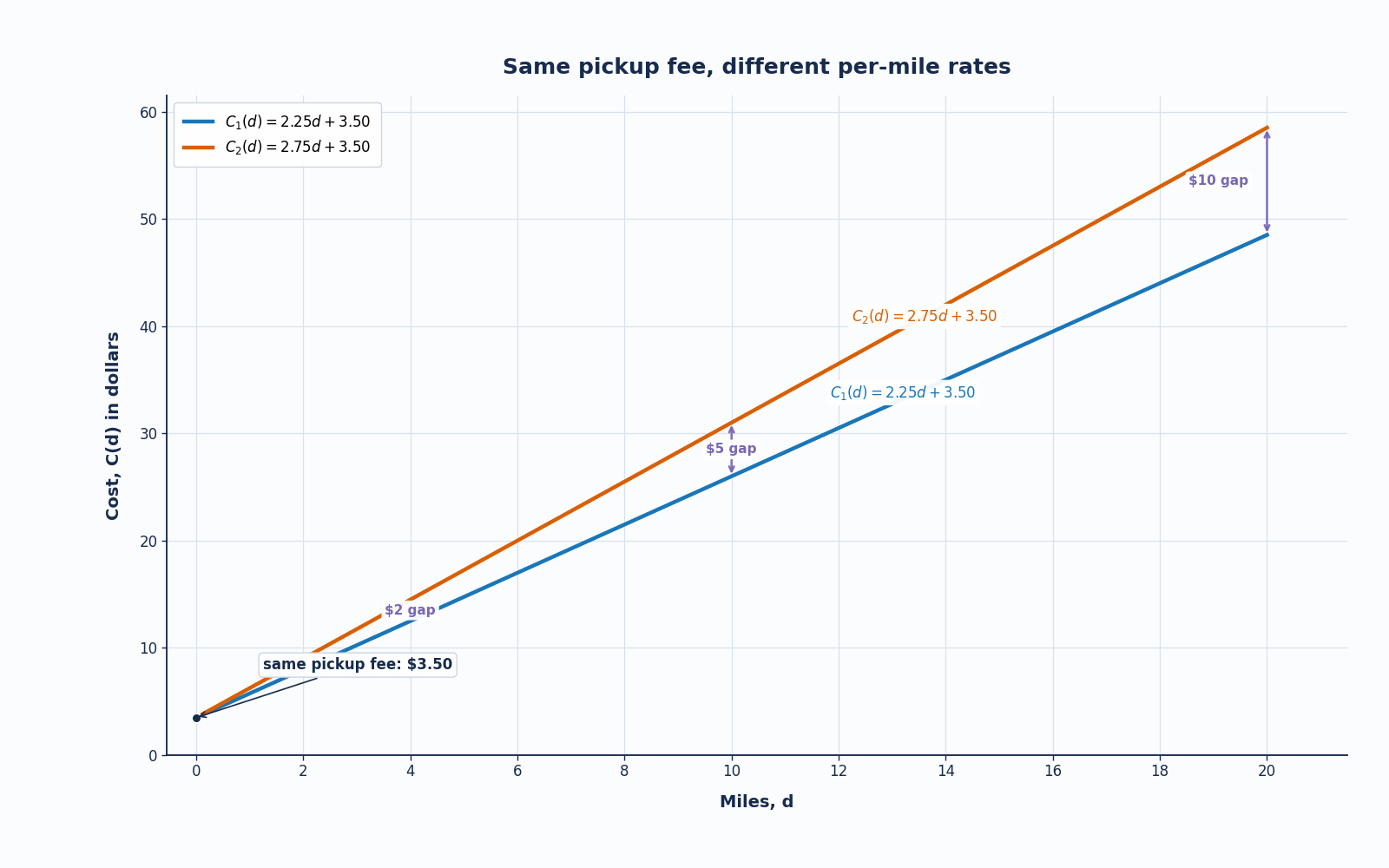
Now take two models that begin at the same place but climb at different rates, y1=m1x+b and y2=m2x+b. Subtracting one from the other, the shared starting value cancels and leaves something remarkably simple:
g(x)=y2−y1=(m2−m1)x
The gap is itself a line through the origin. It starts at zero and grows in direct proportion to the input, which means a rate change never produces a fixed difference: double the input and the gap doubles; multiply the input by ten and the gap multiplies by ten.
Here are two taxi models, both keeping the $3.50 pickup fee, at $2.25 and $2.75 per mile:
Miles d
C1=2.25d+3.50
C2=2.75d+3.50
Gap
0
$3.50
$3.50
$0.00
4
$12.50
$14.50
$2.00
10
$26.00
$31.00
$5.00
20
$48.50
$58.50
$10.00
Every gap matches (2.75−2.25)d=0.50d, and the graph below turns that column into a widening wedge between the two lines.
Short rides barely notice the increase, while long rides absorb almost all of it — the same "distance from the pivot" effect from the last lesson, now measured in dollars.
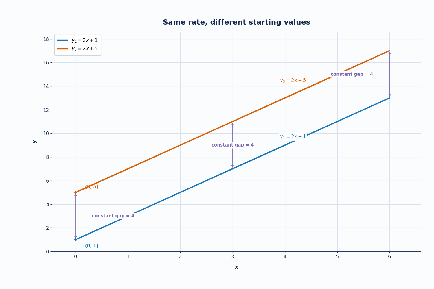
Change the starting value instead, and the arithmetic goes the other way. With y1=mx+b1 and y2=mx+b2, the shared rate cancels:
g(x)=y2−y1=b2−b1
No x survives in the result, so the gap is the same forever. On a graph the two lines are parallel: one sits above the other by a constant vertical distance, no matter how far right we look. This is the vertical shift from the first course of the path, seen now from a comparison angle.
The contrast between the two cases is the heart of the diagnosis. A rate change opens the lines apart like a pair of scissors, while a starting-value change slides one line up or down without ever touching the spacing.
Graphs are convenient, but data usually arrives as a table, so let us run the same diagnosis on numbers. Two steps do the whole job: read the output at x=0 to get the starting value, then divide the change in output by the change in input between two rows to get the rate, m=ΔxΔy.
x
Model A
Model B
0
12
12
2
18
22
4
24
32
6
30
42
Both models start at 12, so the starting value is untouched. Model A rises by 6 every 2 steps, giving mA=3, while Model B rises by 10 every 2 steps, giving mB=5. The rate changed, from 3 to 5, and the gaps read 0,4,8,12 — growing by 2 per unit of x, exactly as (5−3)x predicts.
One warning before you try this yourself: if the table does not include x=0, do not guess at the starting value. Find the rate first and step backwards. A model reading 20 at x=2 with a rate of 3 has a starting value of 20−2⋅3=14.
Suppose a streaming service charges $8 per month with a $15 activation fee, so Cold(t)=8t+15. The new plan announces $11 per month with the same $15 activation, giving Cnew(t)=11t+15.
The activation fee is identical, so the starting value did not move; only the rate did, from $8 to $11 per month. The gap is therefore (11−8)t=3t dollars: $3 after one month, $18 after six months, and $36 after a full year.
Saying "the price went up by $3" is true only for the very first month. That is the mistake this lesson exists to prevent — a rate change costs more the longer we stay.
Every linear model holds a rate m and a starting value b, and the units tell us which is which. When two models share a starting value, their gap is (m2−m1)x and widens steadily with the input; when they share a rate, their gap is the constant b2−b1. To diagnose any change, compare intercepts and signed rates — reading them straight off a graph, or recovering them from a table using the output at x=0 and the step size between rows.
That completes Slope Changes and Rates of Change, and the diagnosis is now yours to run. In the exercises ahead you will pick out rates and starting values from pay slips and fares, build a gap table row by row, match observable signatures to their conclusions, and pull both numbers out of raw data. Your final task puts a real gym price change in front of you, where you will name what moved, back it with specific numbers, and explain what it costs over a full year.