Scaled Dot-Product Attention and Masking in Transformers
Introduction
Welcome back to our journey through "Sequence Models & The Dawn of Attention"! We've made excellent progress, and I'm excited to dive deeper with you into lesson 3. In our previous lessons, we witnessed the limitations of traditional RNNs and LSTMs when handling long sequences, then discovered how attention mechanisms like Luong and Bahdanau elegantly solve the fixed-context bottleneck by enabling selective focus on different parts of input sequences.
Today, we're taking a crucial step toward the Transformer architecture by exploring scaled dot-product attention, the foundational attention mechanism that powers modern language models like GPT and BERT. We'll understand why the scaling factor is mathematically essential, then dive deep into masking techniques that are absolutely critical for real-world applications. Masking isn't just a technical detail; it's what enables models to ignore padding tokens and maintain the autoregressive property that makes language generation possible. Let's build this understanding step by step!
Understanding the Scaling Factor
Implementing Scaled Dot-Product Attention
The Critical Role of Masking
Padding Masks: Ignoring Irrelevant Tokens
Let's implement padding masks to handle sequences of different lengths. Padding masks ensure our model doesn't waste attention on meaningless padding tokens:
The create_padding_mask function creates a boolean mask where True indicates real tokens and False indicates padding tokens. We use pad_idx=0 as our padding token identifier. The unsqueeze(1) operation adds a dimension to make the mask broadcastable with attention scores. In create_sample_sequences, we create realistic sample data where the first sequence has length 4 (positions 4 - 5 are padded with zeros), and the second sequence uses the full length of 6. This simulates the common scenario where sequences in a batch have different natural lengths but need to be padded to the same size for efficient processing.
Now let's bring everything together and see how different masking strategies affect attention patterns. We'll test our scaled dot-product attention with various mask combinations:
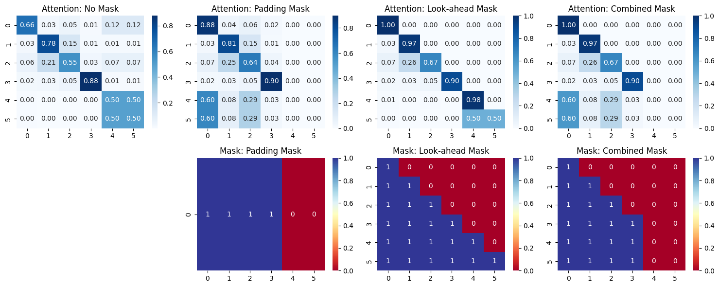
To better understand how our masking strategies affect attention behavior, let's implement a comprehensive visualization function that displays both attention weights and the masks that shape them:
Python
def visualize_attention_and_masks(attention_weights, masks, titles):
    """Visualize attention weights and masks"""
    fig, axes = plt.subplots(2, len(titles), figsize=(15, 6))

    # Plot attention weights
    for i, (attn, title) in enumerate(zip(attention_weights, titles)):
        sns.heatmap(attn[0].detach().numpy(), annot=True, fmt='.2f',
                   cmap='Blues', ax=axes[0, i])
        axes[0, i].set_title(f'Attention: {title}')

    # Plot masks
    for i, (mask, title) in enumerate(zip(masks[1:], titles[1:])):
        i += 1 # skip first plot
        if mask is not None:
            if mask.dim() == 3:
                mask_viz = mask[0].float()  # Take first batch item
            elif mask.dim() == 2:
                mask_viz = mask.float()  # Already 2D
            else:
                raise ValueError(f"Unexpected mask dimension: {mask.dim()}")
            sns.heatmap(mask_viz.numpy(), annot=True, fmt='.0f',
                       cmap='RdYlBu', ax=axes[1, i])
            axes[1, i].set_title(f'Mask: {title}')

    fig.delaxes(axes[1, 0])
    plt.tight_layout()
    plt.savefig("plot.png")
This visualization function creates a dual-row layout that reveals the relationship between masks and resulting attention patterns. The top row displays attention weight heatmaps, where darker blue indicates stronger attention connections between positions. The bottom row shows the corresponding mask matrices, where blue (1) indicates allowed attention and red (0) indicates blocked attention.
The function handles the dimensional complexity of our masks elegantly. Since padding masks have shape (batch_size, 1, seq_len) while look-ahead masks have shape (seq_len, seq_len), we need to extract the appropriate 2D matrix for visualization. Notice how we skip the first mask plot (using fig.delaxes(axes[1, 0])) since the "no mask" scenario has no mask to display.
Interpreting Attention and Mask Visualizations
Now let's call this function in main to test and visualize the different masking scenarios:
When we examine the resulting visualization, several critical patterns emerge:
The "no mask" attention shows the model freely attending to all positions, including meaningless padding tokens.
The "padding mask" properly zeros out attention to padded positions (columns 4-5 for the first sequence), which ensures positions don't attend to padding tokens.
The "look-ahead mask" creates the distinctive lower-triangular pattern essential for autoregressive generation, enforcing causality.
Most importantly, the "combined mask" demonstrates how both constraints work together, creating the exact attention pattern needed for real-world language modeling where we must respect both padding boundaries and causal ordering.
This systematic comparison reveals how each masking strategy shapes attention behavior.
Be a part of our community of 1M+ users who develop and demonstrate their skills on CodeSignal
The scaling factor of dk1 is mathematically necessary to avoid crippling our attention mechanism. When we compute attention scores using dot products between queries and keys, the magnitude of these scores grows with the dimensionality dk of our vectors. If we have high-dimensional vectors (say, dk=512 or dk=1024 as in real Transformers), the dot products can become very large. This creates a problem when we apply the softmax function: large input values to softmax result in extremely sharp probability distributions, where one element gets almost all the weight (approaching 1) and others get nearly zero weight.
This sharp distribution has devastating effects on gradients during backpropagation. The softmax function's gradient becomes vanishingly small in regions where the output is close to 0 or 1, leading to the vanishing gradient problem. By scaling the dot products by dk1, we keep the variance of the attention scores roughly constant regardless of the dimensionality, ensuring that softmax operates in a regime where gradients remain healthy and learning can proceed effectively.
Masking in attention mechanisms serves two fundamental purposes that are absolutely essential for practical applications. Without proper masking, our models would either attend to meaningless padding tokens or violate the causal structure required for language generation.
The first challenge arises from padding tokens. In practice, we batch sequences of different lengths together for efficient processing, padding shorter sequences with special tokens (usually zeros) to match the longest sequence in the batch. Without masking, our attention mechanism would treat these padding tokens as legitimate parts of the input, potentially learning to focus on meaningless information and degrading performance.
The second challenge involves autoregressive generation, the foundation of language models like GPT. During training and inference, the model must generate tokens one at a time, with each position only allowed to attend to previous positions. This prevents the model from "cheating" by looking ahead to future tokens during training. Without this look-ahead masking (also called causal masking), the model would learn an unrealistic mapping that couldn't be replicated during actual generation.
Both masking types work by setting certain attention scores to very large negative values (like -1e9) before applying softmax. Since softmax(−∞)=0, these positions effectively receive zero attention weight.
Today we've built a solid foundation in scaled dot-product attention and masking, two absolutely critical components of the Transformer architecture. We discovered why the scaling factor dk1 is mathematically essential for preventing gradient issues, and we implemented comprehensive masking strategies that handle real-world challenges. The padding and look-ahead masks we created aren't just implementation details; they're fundamental to how modern language models like GPT work.
In our next lesson, we'll build upon these foundations to explore multi-head attention, discovering how parallel attention mechanisms can capture different types of relationships simultaneously. This will bring us even closer to understanding the full Transformer architecture, and the masking techniques we've learned today will become even more important as we scale up to multiple attention heads working in parallel!
Let's implement the scaled dot-product attention mechanism, which forms the core of the Transformer architecture. This mechanism combines the efficiency of dot-product similarity with the mathematical stability provided by the scaling factor:
This implementation follows the mathematical formula: Attention(Q,K,V)=softmax(dkQKT)V. We compute the dot products between queries and keys, apply the crucial scaling factor, optionally apply masking (we'll explore this next), then use softmax to convert scores into attention weights. Finally, we compute the weighted sum of values using these attention weights. Notice how the mask parameter allows us to selectively ignore certain positions, which is essential for handling padding tokens and implementing causal attention for language modeling.
Look-ahead masking is crucial for autoregressive models, ensuring each position can only attend to previous positions. This maintains the sequential nature of language generation:
The create_look_ahead_mask function uses torch.triu (upper triangular) to create a mask matrix. The diagonal=1 parameter means we start the upper triangular part from the diagonal above the main diagonal, effectively creating a lower triangular mask when we invert it with mask == 0. This results in a boolean mask where each position i can attend to positions 0 through i (inclusive), but not to positions i+1 and beyond.
For a sequence of length 4, this creates a mask pattern like:
Position 0: can attend to [0]
Position 1: can attend to [0, 1]
Position 2: can attend to [0, 1, 2]
Position 3: can attend to [0, 1, 2, 3]
This structure is essential for language modeling, where predicting the next token should only depend on previously generated tokens, not future ones.