Welcome back! You have already accomplished a lot in your machine learning journey. So far, we have revisited how to explore and prepare data, train a linear regression model, and save our trained model for future use. In this lesson, we will take the next important step: evaluating our trained model’s performance on new, unseen data — the test set.

Evaluating our model on test data is crucial because it tells us how well our model is likely to perform in the real world, not just on the data it has already seen. By the end of this lesson, you will know how to load our test data and trained model, make predictions on the test set, calculate key evaluation metrics, and visualize our model’s performance. These skills are essential for any machine learning practitioner and will help you build models that generalize well to new situations.

The first thing we need to do is load the test data and the trained model. The test data contains the same features as the training data, and the target variable is still MedHouseVal. To use our trained model, we will load it from the file where we saved it using the joblib library.

Here is how we can do this:

In this code, we first load the test data and separate the features (X_test) from the target variable (y_test). Then, we load the trained model from the file trained_model.joblib. This prepares us to make predictions on new data.

With the test data and trained model loaded, we are ready to make predictions. This is a key moment: we are now using our model to predict house values for data it has never seen before. This step shows how our model might perform in real-world scenarios.

To make predictions, we simply call the predict method of our model and pass in the test features. Here is how we do it:

After running this code, y_pred will contain the predicted median house values for each sample in the test set. This is the first time our model is being tested on truly unseen data, which is why this step is so important.

Now that we have predictions, it is time to measure how well our model performed. There are several metrics we can use to evaluate regression models. In this lesson, we will focus on four key metrics:

• Mean Squared Error (MSE): This measures the average squared difference between the predicted and actual values. Lower values are better.
• Root Mean Squared Error (RMSE): This is the square root of MSE and is in the same units as the target variable, making it easier to interpret.
• Mean Absolute Error (MAE): This measures the average absolute difference between the predicted and actual values. Like RMSE, lower values are better.
• R² Score: This tells us how much of the variance in the target variable is explained by our model. Values closer to 1 mean better performance.

Here is how we can calculate these metrics using Scikit-Learn:

When we run this code, we will see output like the following:

These numbers tell us how close our model’s predictions are to the actual values in the test set. For example, an RMSE of 0.68 means that, on average, our predictions are about 0.68 units away from the true values. An R² score of 0.6456 means our model explains about 64.56% of the variance in house values on the test set.

Numbers are helpful, but sometimes a picture can make things even clearer. One common way to visualize regression model performance is to plot the actual values against the predicted values. If our model is perfect, all points will fall on a straight line (the reference line) where the predicted value equals the actual value.

Here is how we can create this plot using matplotlib:

This code creates a scatter plot where each point represents a test sample. The x-axis shows the actual house values, and the y-axis shows the predicted values. The red dashed line is the reference line where predictions would be perfect. The closer the points are to this line, the better our model is performing.

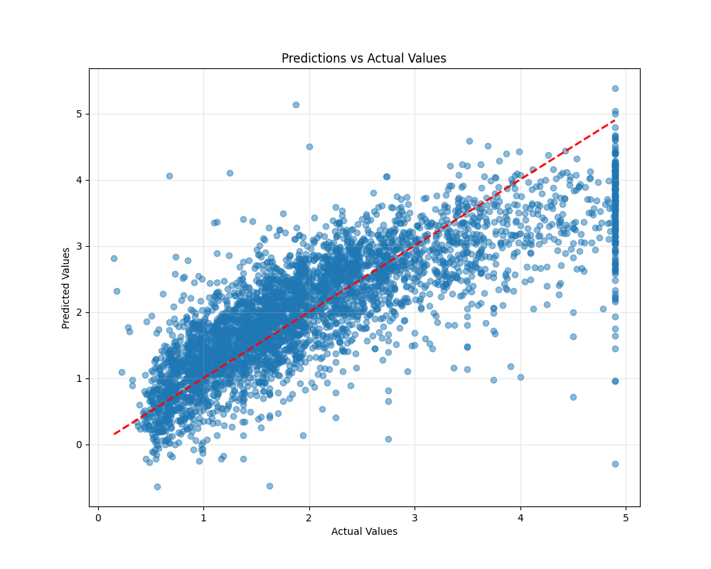
By looking at this plot, we can quickly see whether our model tends to overestimate or underestimate values, or if there are any patterns in the errors.

In this lesson, you learned how to evaluate our trained linear regression model on the test set. We loaded the test data and the saved model, made predictions on unseen data, calculated important evaluation metrics, and visualized our model’s performance. These steps are essential for understanding how well our model generalizes to new data and for identifying areas where it might need improvement.

You are now ready to move on to practice exercises, where you will apply these skills and deepen your understanding. Keep up the great work — each lesson brings us closer to building reliable and effective machine learning models!