Question Evidence from Small Samples
Introduction 🎉
Welcome to Question Evidence from Small Samples! Over the previous four lessons you learned how independent events behave, saw why the gambler's fallacy and hot-hand belief mislead us, used regression to the mean to interpret extreme performances, and discovered why randomness naturally produces clusters, coincidences, and false patterns. All of those ideas share a common thread: random processes create surprising-looking outcomes far more often than we expect. In this final lesson, you'll turn to one of the most practical applications of that insight. By the end of this lesson, you will have learned to:
- Explain why small samples produce extreme and unstable results, and recognize that randomness has not had enough observations to settle down when the data is limited.
- Convert percentages back into raw counts to expose thin evidence, and always ask "out of how many?" before trusting a number.
- Apply practical evaluation questions about sample size, actual counts, and replication to decide whether a trend or difference is genuine or just noise from limited data.
These skills are essential for clear thinking in a world full of data. By mastering these concepts, you will learn to pause before trusting a number and recognize when an apparent signal is really just noise from too little evidence.
The Problem With Small Amounts of Evidence 🌱
Imagine two restaurants on the same street. Restaurant A has a 4.9-star rating based on 7 reviews. Restaurant B has a 4.4-star rating based on 1,200 reviews. Which one is actually better?
Most of us are drawn to the higher number, but that 4.9 rating is standing on very thin ground. With only 7 opinions, a single unhappy diner could drop the average dramatically. Restaurant B's rating, built on over a thousand experiences, is far more stable. This everyday example captures the core lesson: the less data behind a number, the less that number tells us.
Randomness produces streaks, clusters, and extreme results all the time, as we saw throughout this course. Small samples are where those effects hit hardest, because there simply is not enough data for the extremes to balance out.
Let's make this concrete with a simple thought experiment. Suppose a fair coin is flipped repeatedly and we record the percentage of heads.
- In 10 flips, getting 80% heads (8 out of 10) is unusual but not shocking.
- In 100 flips, getting 80% heads (80 out of 100) is virtually impossible with a fair coin.
- In 1,000 flips, the percentage of heads will almost certainly land between 47% and 53% — the result barely strays from 50% because the large sample leaves randomness very little room to push it around.
The pattern is clear: the smaller the sample, the wilder the results. This is not a flaw in the data collection; it is a basic property of randomness. Small samples simply have not run long enough for that settling to occur.
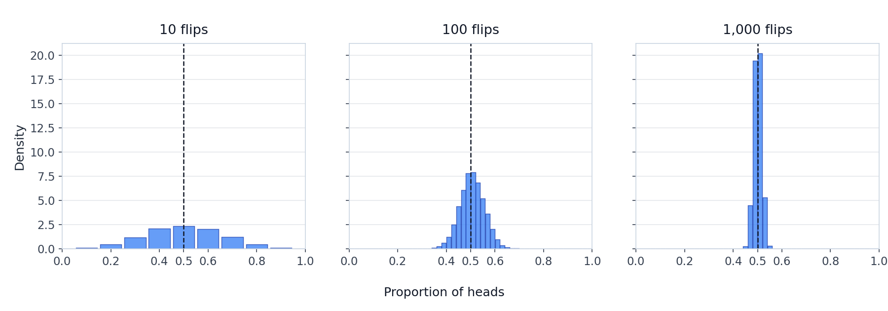
Notice why this happens. In a small sample, a single observation carries enormous weight — flipping just one or two coins the other way swings the percentage wildly. In a large sample, each observation is only a tiny slice of the whole, so no single outcome can move the result very far. That is the heart of why small samples are so unstable: there is simply too little data for the extremes to cancel out.
Percentages Can Hide Thin Evidence 🤏
One of the easiest traps to fall into is taking a percentage at face value without asking how many observations produced it. Consider these three claims:
| Claim | Actual count |
|---|---|
| "80% of users recommend this app" | 4 out of 5 users |
| "Crime jumped 50% this month" | 3 incidents vs. 2 last month |
| "Survey: 67% support the new policy" | 10 out of 15 respondents |
Each percentage sounds decisive. But once you see the raw numbers, the picture changes. A single extra opinion, one more crime, or a couple of different survey answers would shift the percentage dramatically.
A good habit is to convert percentages back into counts whenever possible. If a report says "75% of patients improved," ask: 75% of how many? If the answer is 8 patients, that means 6 improved and 2 did not. One patient switching categories would change the result to 62.5% or 87.5%. The percentage is not wrong, but it gives a false sense of precision that the small sample cannot support.
Suppose two sales teams are compared after one month. Team A closed 60% of their deals (12 out of 20). Team B closed 45% of theirs (90 out of 200). A manager might conclude that Team A has a better strategy, but look at how much each result depends on its sample size.
Start by asking out of how many? Team A's impressive 60% rests on just 20 deals. If only two of those deals had gone the other way, their rate would drop from 60% to 50%, wiping out most of the gap. Team B's 45% rests on 200 deals, so a single different outcome barely moves the number at all.
Because Team A's result is built on so few deals, randomness has a lot of room to push it around. The 15-point gap might reflect a genuinely better strategy or it might just be the natural wobble of a small sample. With only 20 deals, you cannot tell the two apart yet.
The key takeaway: when sample sizes differ, the smaller sample's result is less trustworthy, even if its numbers look more impressive. Before concluding that one group genuinely outperforms another, check whether each result rests on enough observations to be stable.
Spotting Noise Disguised as Trends 🎭
Small samples do not just distort one-time comparisons — they also create the illusion of trends over time. A small town with 4 burglaries one month and 8 the next has seen a "100% increase in crime," but with numbers that low, the jump could easily be random variation. A city logging 400 and 410 burglaries over the same months shows a much smaller percentage change, yet because the counts are large, even that modest shift might be more meaningful.
When you encounter a trend or difference built on limited data, run through these questions:
- How large is the sample? Smaller samples produce larger swings by nature.
- What are the actual counts behind the percentages? Convert rates back to raw numbers whenever possible.
- How much would the result change if just one or two observations were different? In a small sample, a single flip can swing the percentage dramatically; in a large one, it barely registers.
- Has the trend persisted over multiple periods? A pattern that repeats across several independent samples is far more convincing than a single dramatic swing.
These questions connect directly to the evaluation toolkit from the previous lesson where you asked whether a pattern was predicted in advance, how many comparisons were made, and whether it replicated in new data. Here, you add one more question: is the sample big enough for the result to rise above random noise?
Conclusion and Next Steps
In this final lesson, you explored why small samples deserve extra skepticism. Small samples produce extreme and unstable results because randomness has not had enough observations to settle down, and percentages can disguise thin evidence until you convert them back to raw counts. Asking "out of how many?" and trusting repeated evidence over a single dramatic result give you practical ways to judge whether a trend or difference is likely genuine or just noise from limited data.
The practice exercises ahead will bring everything together. You will watch small and large samples behave side by side, unpack percentages into real counts, weigh competing claims, evaluate suspicious trends, and challenge someone's bold conclusion built on too little evidence. Jump in and see how sharp your new toolkit really is!
