Customer Spend Quartiles

Welcome to Lesson 4 of 4 in Ranking with RANK, DENSE_RANK, and ROW_NUMBER. We have already selected first customer orders, compared tied rankings, and found leading products within categories. In this final lesson, we will move from ranking individual results to organizing every customer into a useful order-value segment.

We will calculate each customer’s gross total order value, assign all 50 customers to four approximately equal row buckets with NTILE(4), and treat quartile 1 as the highest-value group. Because the query does not filter order_status, canceled and refunded orders remain included in the calculation.

One modelling note before we calculate money. OrderItems records what was bought and how many, but not the price paid at the time, so these reports reconstruct historical value from the current Products.product_price. A production schema would capture a transaction-time unit price on the order line, because catalog prices change. In this dataset prices are assumed to be immutable, and the current price is used as a deliberate proxy.

Before assigning quartiles, we need one comparable row for each customer. As we learned when building CTE pipelines, the first stage should establish a clear grain for the next calculation. The customer_order_value CTE follows the relationships from customers to orders, order items, and products, then sums quantity * product_price.

WITH customer_order_value AS (
    SELECT
        c.customer_id,
        c.customer_name,
        SUM(oi.quantity * p.product_price) AS gross_order_value
    FROM Customers AS c
    INNER JOIN Orders AS o
        ON o.customer_id = c.customer_id
    INNER JOIN OrderItems AS oi
        ON oi.order_id = o.order_id
    INNER JOIN Products AS p
        ON p.product_id = oi.product_id
    GROUP BY
        c.customer_id,
        c.customer_name
)

The joins connect each order item to its product price and its customer. Grouping by the customer identifier and name produces one row per customer. The internal alias gross_order_value represents the gross total order value for each customer. Since there is no order_status condition, every matching order contributes, including canceled and refunded orders.

A window function assigns results to the rows produced by its source query. If we applied NTILE(4) directly to OrderItems, customers with many line items would appear repeatedly, and the buckets would classify order items instead of customers. Starting from Orders would still repeat customers who placed multiple orders.

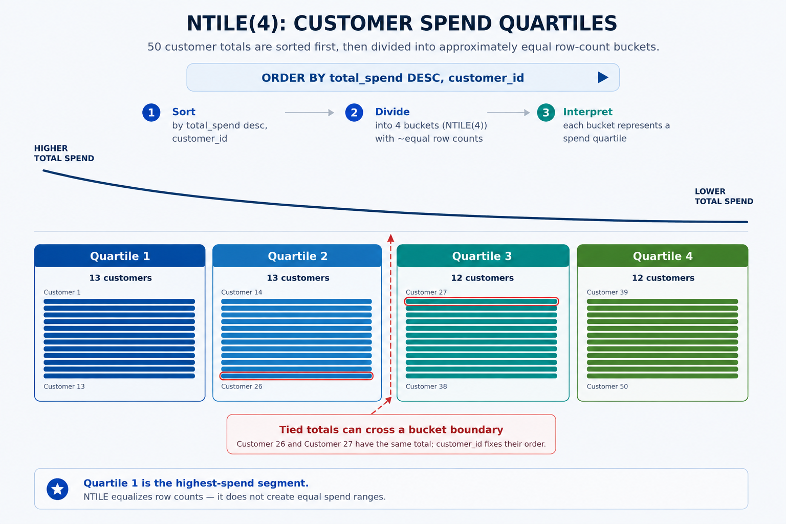
The CTE prevents both problems by reducing $quantity \times product\_price$ to one customer total before segmentation. Because the dataset contains 50 customers, the four buckets will contain approximately 13, 13, 12, and 12 rows. These are equalized row counts, not equal ranges of order value, so tied totals can appear on opposite sides of a bucket boundary.

Now that the input contains one row per customer, we can apply NTILE(4). We order by total order value in descending order, placing the highest-value rows first. The customer identifier then provides a unique, stable tiebreaker. This differs from our use of RANK() and DENSE_RANK(), where adding an identifier would destroy meaningful ties.

WITH customer_order_value AS (
    SELECT
        c.customer_id,
        c.customer_name,
        SUM(oi.quantity * p.product_price) AS gross_order_value
    FROM Customers AS c
    INNER JOIN Orders AS o
        ON o.customer_id = c.customer_id
    INNER JOIN OrderItems AS oi
        ON oi.order_id = o.order_id
    INNER JOIN Products AS p
        ON p.product_id = oi.product_id
    GROUP BY
        c.customer_id,
        c.customer_name
)
SELECT
    customer_id,
    customer_name,
    gross_order_value,
    NTILE(4) OVER (
        ORDER BY gross_order_value DESC, customer_id
    ) AS order_value_quartile
FROM customer_order_value

NTILE(4) returns bucket numbers from 1 through 4. Since the ordering is descending, bucket 1 contains the highest total order values. We do not use PARTITION BY because all customers belong to one segmentation population. The customer ID makes assignments repeatable, but equal totals can still be split when a bucket boundary falls within a tie.

The final query keeps the raw total order value for ordering and bucket assignment, then rounds it for display. The report alias gross_order_value describes the metric more precisely than “revenue” because canceled and refunded orders remain included. Similarly, order_value_quartile identifies the quartile based on the customer’s total order value.

The outer ORDER BY uses the same descending value order as NTILE(4), followed by ascending customer ID. This makes both the bucket assignments and displayed rows deterministic.

WITH customer_order_value AS (
    SELECT
        c.customer_id,
        c.customer_name,
        SUM(oi.quantity * p.product_price) AS gross_order_value
    FROM Customers AS c
    INNER JOIN Orders AS o
        ON o.customer_id = c.customer_id
    INNER JOIN OrderItems AS oi
        ON oi.order_id = o.order_id
    INNER JOIN Products AS p
        ON p.product_id = oi.product_id
    GROUP BY
        c.customer_id,
        c.customer_name
)
SELECT
    customer_id,
    customer_name,
    ROUND(gross_order_value, 2) AS gross_order_value,
    NTILE(4) OVER (
        ORDER BY gross_order_value DESC, customer_id
    ) AS order_value_quartile
FROM customer_order_value
ORDER BY gross_order_value DESC, customer_id;

This single MySQL 8.0 statement first creates customer-level totals, then assigns deterministic quartiles, and finally formats and orders the report. Rounding affects presentation only. The raw value remains available for the window ordering, so customers are not repositioned because of rounded display values.

We have completed the ranking course by building a customer segmentation report with NTILE(4). First, we joined the related tables and aggregated order item values into one total order value per customer. Next, we assigned customers to four approximately equal row buckets, with quartile 1 representing the highest-value segment. Finally, we rounded the displayed values and used customer ID to keep both bucket assignments and report ordering stable.

Remember that NTILE creates row buckets, not equal value bands. Unlike RANK() and DENSE_RANK(), it does not preserve shared ranking positions for ties. A deterministic tiebreaker is therefore useful, but tied customers may still be placed in different quartiles.

Congratulations on reaching the end of Ranking with RANK, DENSE_RANK, and ROW_NUMBER. In the upcoming practice section, we will inspect the source data, build the customer total order value calculation, assign quartiles, and complete the stable report one step at a time.