Welcome to the first lesson of PredictHealth's Multi-Factor Cost Models course. In this lesson, you will learn how to analyze and predict insurance costs using combined factor analysis. Combined factor analysis means looking at more than one variable at a time to understand how they work together to affect insurance costs. This approach is at the heart of PredictHealth's cost modeling, where we use real-world data to make better predictions and decisions.
By the end of this lesson, you will know how to build a simple multiple regression model using two important factors — age and BMI — to predict insurance charges. You will also learn how to interpret the results, evaluate the model's performance, and visualize the predictions. This lesson will give you a strong foundation for more advanced cost modeling techniques later in the course.
Let's start by understanding the insurance dataset we will use. The insurance dataset contains information about individuals, including their age, sex, BMI (Body Mass Index), number of children, smoking status, region, and the insurance charges they paid. Here is a quick look at what the data might look like:
| age | sex | bmi | children | smoker | region | charges |
|---|---|---|---|---|---|---|
| 19 | female | 27.9 | 0 | yes | southwest | 16884.92 |
| 18 | male | 33.8 | 1 | no | southeast | 1725.55 |
| 28 | male | 33.0 | 3 | no | southeast | 4449.46 |
In this lesson, we will focus on two numerical features: age and bmi. These are important because age often affects health risks, and BMI is a common measure of body fat, which can also impact health and insurance costs. While there are other features in the dataset, starting with these two helps us build a clear and simple model.
Before we can build a model, we need to prepare the data. First, let's import all the necessary libraries:
Next, we need to separate the features (the variables we use to predict) from the target (the value we want to predict, which is charges). We also need to split the data into a training set and a testing set. The training set is used to build the model, and the testing set is used to see how well the model works on new data.
Here is how you can do this in Python:
While age (typically 18-65 years) and BMI (typically 15-50) are on similar scales in our dataset, it's important to know when standardization is needed. Standardization (scaling variables to have mean 0 and standard deviation 1) is recommended when features have very different scales (e.g., age vs. income in dollars), when using regularized models (Ridge, Lasso), when using distance-based algorithms, or when coefficients need to be directly compared for importance. In our case, since both features are on comparable scales, standardization is optional, but it's good practice to consider it for more robust modeling.
Before building our model, it's crucial to understand that multiple regression relies on several key assumptions. Violating these assumptions can lead to unreliable results:
Linearity: The relationship between predictors and the target should be linear. We can check this by plotting each feature against the target variable.
Independence: Observations should be independent of each other. This is usually satisfied if data is collected properly without time dependencies or clustering.
Homoscedasticity (Constant Variance): The variance of residuals should be constant across all levels of predicted values. We check this with residual plots.
Normality of Residuals: Model residuals should be approximately normally distributed. This can be checked with Q-Q plots or histogram of residuals.
No Multicollinearity: Predictor variables shouldn't be highly correlated with each other. We can check this using correlation matrices or Variance Inflation Factor (VIF).
Understanding these assumptions is important for building reliable models. In practice, you would check these assumptions after building your model, but knowing them upfront helps you make better modeling decisions.
Now that the data is ready, let's build a regression model that uses both age and bmi to predict insurance charges. This is called a multiple regression model because it uses more than one feature.
Here is the code to create and train the model:
By combining age and bmi, the model can capture more information about what affects insurance costs. This usually leads to better predictions than using just one factor.
After building the model, it's important to check how well it works. We use several metrics for this:
- Mean Squared Error (MSE): Measures the average squared difference between actual and predicted values.
- Root Mean Squared Error (RMSE): The square root of MSE, which brings the error back to the original units (dollars).
- R-squared (R²): Shows how much of the variation in insurance charges is explained by the model.
Let's look at the code and the output:
Example output might look like this:
The coefficients tell us how much the insurance cost changes for each unit increase in age or bmi. For example, if the age coefficient is 223.80, then for each additional year of age, the insurance cost increases by about $223.80, holding BMI constant. Similarly, for each unit increase in BMI, the cost increases by $330.79.
This kind of interpretation is very useful for business decisions. It helps insurance companies understand how much each factor contributes to the overall cost.
A good way to see how well the model is working is to plot the predicted insurance charges against the actual charges. This helps us spot patterns and see if the model is making reasonable predictions.
Here is how you can create the plot:
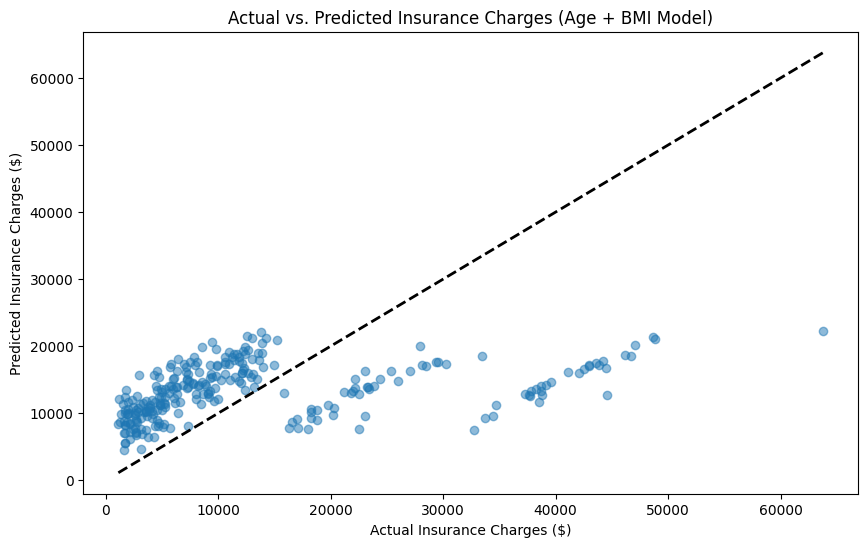
Interpreting the Plot: The diagonal line represents perfect predictions (predicted = actual). Points clustered close to this line indicate good predictions, while points scattered far from the diagonal suggest prediction errors. The spread around the line indicates the model's overall accuracy. In our example plot, you can see that most points follow the general trend of the diagonal line with some scatter, which is normal and expected. A few outliers exist where the model significantly under- or over-predicts, and the overall pattern suggests the model captures the basic relationship but has room for improvement.
Good model signs include points clustered close to the diagonal line, while poor model signs include points scattered far from the diagonal, wide spread, or systematic patterns away from the line. The R² value of 0.15 tells us that our model explains about 15% of the variance in insurance charges using just age and BMI. While this is modest, it's a good starting point that can be improved by adding more relevant features.
In this lesson, you learned how to use combined factor analysis to predict insurance costs. You explored the insurance dataset, selected important features, prepared the data, understood key regression assumptions, built a multiple regression model, evaluated its performance, and visualized the results. You also learned how to interpret the model's coefficients in a business context and check important model assumptions.
You are now ready to practice these skills with hands-on exercises. In the next part of the course, you will get to apply what you have learned and explore more advanced modeling techniques. Great job completing this lesson — keep up the good work!
