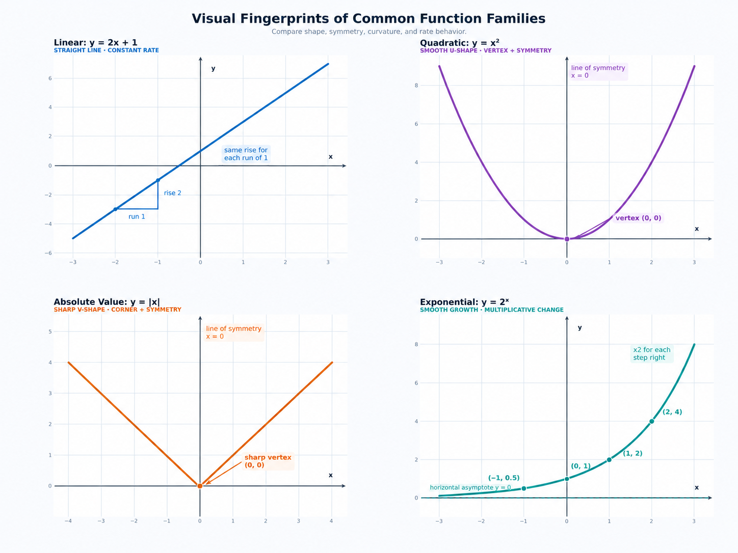
Imagine receiving a graph with its equation hidden. Before calculating any points, you can often predict the kind of rule behind it by noticing whether the graph bends smoothly, changes direction at a corner, or becomes steeper through repeated multiplication.
This is the first lesson in Nonlinear Graphs and Key Features. Building on your earlier work with coordinates, functions, and lines, you will learn to recognize the visual fingerprints of three nonlinear families: quadratic, absolute-value, and exponential functions.
By the end of this lesson, you will be able to:
Distinguish a linear graph from a nonlinear graph.
Recognize quadratic, absolute-value, and exponential graphs.
Use shape, symmetry, curvature, and rate behavior as evidence.
Confirm a function family from an equation, table, or real-world description.
Why Graphs Have Visual Fingerprints
A function connects an input x to an output y, often written as y=f(x). The way the output responds when the input changes determines the graph’s shape.
For a linear rule such as y=3x+1, every increase of 1 in x adds 3 to y. This constant additive change creates a straight line. In contrast, y=x2 produces the outputs 0, 1, 4, and 9 for x=0, 1, 2, and 3; the changes are 1, then 3, then 5, so the graph bends.
A function family is a group of functions with a shared basic pattern. A shift, stretch, or reflection may change a graph’s location or direction, but the family’s main fingerprint remains. For example, every quadratic has a smooth parabolic pattern, even when its vertex is not at the origin.
Quadratic Functions: Smooth Parabolas
The first nonlinear family to recognize is the quadratic family. A quadratic function contains a squared variable and can be written as
y=ax2+bx+c,a=0
The simplest example is y=x2. Its values form this table:
x
−2
−1
0
1
2
y=x2
4
1
0
1
4
The equal outputs for inputs equally far from 0 reveal symmetry about the y-axis. The points form a smooth, bowl-shaped curve called a parabola, and the bottom point is its vertex.
A quadratic can also be written in vertex form:
y=a(x−h)2+k
In this form, the vertex is (h,k) and the graph is symmetric about the vertical line x=h. If a>0, the parabola opens upward and has a minimum; if a<0, it opens downward and has a maximum. The size of ∣a∣ affects how narrow or wide the parabola appears.
Quadratic graphs often model a quantity that rises or falls to one main turning point. For example, the height of a ball thrown into the air can be approximated by a downward-opening parabola: the ball rises, reaches a maximum height, and then falls.
Join the 1M+ learners on CodeSignal
Be a part of our community of 1M+ users who develop and demonstrate their skills on CodeSignal
Absolute-Value Functions: Sharp V Shapes
Exponential Functions: Multiplication Drives The Curve
Compare The Four Function Families
A Reliable Recognition Strategy
Apply The Clues To Examples
Common Mistakes And How To Avoid Them
Key Takeaways
Conclusion And Next Steps
You can now treat a graph’s shape as evidence rather than decoration. A quadratic makes a smooth turn, an absolute-value function makes a sharp corner, and an exponential function changes by a constant multiplier measured from its horizontal asymptote; a line remains the constant-rate reference. Shifts, stretches, and reflections may change position or direction, but they do not erase the family’s fingerprint.
In the practice section, you will classify unfamiliar graphs and equations, explain the clues you used, and use tables or real-world descriptions to confirm your choices. This practice will prepare you to construct quadratic and absolute-value graphs in the next lesson, with exponential graphs revisited in later work.
The absolute value of a number describes its distance from zero. For example, ∣−4∣=4 because −4 is four units from 0. The basic function y=∣x∣ has a sharp V shape with vertex (0,0).
The definition of absolute value explains the two sides of the graph:
∣x∣={x,−x,x≥0,x<0
The right side follows one line and the left side follows a reflected line. They meet at a sudden corner, so the entire graph is not one straight line even though each side is straight.
A transformed absolute-value function has the form
y=a∣x−h∣+k,a=0
Its vertex is (h,k) and its line of symmetry is x=h. A positive value of a creates an upward V, while a negative value creates a downward V. The key clue is the sharp change in direction at the vertex, which is different from the smooth turn of a quadratic.
Absolute-value functions can model distance from a target or location. If a delivery driver is measuring distance from a central warehouse, being two miles east or two miles west may give the same distance. That mirror-image behavior is a useful clue for recognizing absolute value.
An exponential function has the variable in the exponent rather than as a base raised to a fixed power. A common form is
y=abx−h+k,a=0,b>0,b=1
For the basic function y=2x, each increase of 1 in x multiplies the output by 2:
x
−1
0
1
2
y=2x
21
1
2
4
This is a multiplicative pattern, not an additive one. The output changes by larger amounts as the graph rises, even though the multiplying factor stays the same.
The constant ratio between consecutive outputs holds when k=0, that is, when the horizontal asymptote is y=0. If the graph is shifted vertically so that k=0, the outputs themselves no longer have a constant ratio; instead, the distances from the asymptote are multiplied by b at each step:
f(x+1)−k=b(f(x)−k)
For example, y=2x+5 gives the outputs 6, 7, 9, and 13 for x=0, 1, 2, and 3. Those outputs are not in a constant ratio, but subtracting the asymptote value 5 leaves 1, 2, 4, and 8, which double each time. So when you test a table for an exponential pattern, either check the ratios directly (unshifted case) or check the ratios after subtracting the asymptote value (vertically shifted case).
When b>1 and the coefficient is positive, the function shows exponential growth. When 0<b<1, as in y=(21)x, it shows exponential decay. Exponential graphs usually move in one direction without turning around and approach a horizontal line called a horizontal asymptote; for y=2x, that line is y=0, while for y=2x+5 it is y=5.
Exponential functions are useful for modeling repeated percentage change. Compound interest, population growth, and the spread of information can all grow exponentially, while medication leaving the bloodstream or a product losing value may show exponential decay.
The following table places the main families side by side. The linear row provides a reference for identifying the nonlinear patterns.
Family
Common equation signal
Graph fingerprint
Rate behavior
Linear
y=mx+b
Straight line
Constant additive change
Quadratic
An x2 term
Smooth U-shape or upside-down U-shape with a vertex
Additive changes vary smoothly, becoming larger away from the vertex
Absolute value
An expression such as ∣x∣
Sharp V-shape or upside-down V-shape with a vertex
Slope changes suddenly at the corner
Exponential
x appears in an exponent, as in bx
Smooth one-direction curve that approaches a horizontal asymptote
Equal input steps multiply the distance from the asymptote by the same factor
The side-by-side comparison below provides a visual reference for these four families.
A shift, stretch, or reflection can change a graph’s position, width, or direction without changing its family. Therefore, focus on the smoothness of a turn, the presence of a corner, the symmetry, and the rate pattern rather than only on where the graph is located.
When you are given a graph, use the following process:
Scan the overall shape. A straight path suggests a linear function, a smooth bowl suggests a quadratic, a sharp V suggests an absolute-value function, and a one-direction curve suggests an exponential function.
Check how the graph changes direction. A quadratic has a smooth turning point, an absolute-value function has a sharp corner, and an exponential graph usually does not turn around.
Look for symmetry or an asymptote. Mirror-image sides and a vertical line of symmetry favor a quadratic or absolute-value function. A horizontal asymptote is strong evidence of an exponential function.
Compare equal input intervals. The same additive change indicates a linear function, changing additive differences with a smooth turn suggest a quadratic, a sudden slope change suggests absolute value, and a repeated multiplier suggests an exponential function. If the graph or table is shifted vertically, apply the ratio test to the distances from the horizontal asymptote rather than to the outputs themselves.
Confirm with the equation, table, or context. Look for x2, an absolute-value expression, or a variable in an exponent. Use the graph and the equation together when both are available.
If the graph shows only a small portion of a curve, its family may not be obvious. In that situation, an equation, a value table, or information about the real-world situation can provide important confirmation.
Let’s apply the strategy to several equations. The equation gives exact evidence, while the expected graph shape tells us what we should see visually.
Function
Family
Evidence
y=(x−2)2+1
Quadratic
The squared expression creates a smooth upward parabola with vertex (2,1).
y=−∣x+1∣+4
Absolute value
The absolute-value expression creates a corner, and the negative coefficient makes a downward V with vertex (−1,4).
y=3⋅2x
Exponential growth
The variable is in the exponent, and each increase of 1 in x multiplies the output by 2.
y=5(21)x
Exponential decay
The variable is in the exponent, and each increase of 1 in x multiplies the output by 21.
y=2x+5
Exponential growth
The variable is in the exponent; the outputs do not have a constant ratio, but their distances above the asymptote y=5 double with each step.
y=4x−7
Linear
The variable has first power only, so the graph is a straight line with a constant rate.
If you were given only a graph, you could describe its evidence in the same way. For example, a mirror-image graph with a smooth bottom is likely quadratic, while a mirror-image graph with a sharp point is likely absolute value. A curve that rises more and more quickly without turning and approaches a horizontal line is likely exponential growth.
Several quick assumptions can lead to incorrect classifications:
Calling every curved graph exponential. Quadratic graphs also curve. Look for a turning point and symmetry before deciding.
Confusing a quadratic with an absolute-value graph. A quadratic changes direction smoothly, while an absolute-value graph has a sharp corner.
Calling an absolute-value graph linear because its sides are straight. The two sides have different slopes, so the complete graph is not one straight line.
Ruling out an exponential function because the output ratios are not constant. A vertical shift moves the asymptote away from y=0; check the ratios of the distances from the asymptote instead.
Relying only on the y-intercept. Different function families can share the same intercept. Shape and rate behavior provide stronger evidence.
Ignoring shifts and reflections. A downward parabola is still quadratic, and a downward V is still absolute value. The direction may change, but the family remains the same.
Trusting a small graph window too quickly. A limited portion of a graph can hide a vertex or asymptote, so check the equation or a wider range of inputs when possible.
A linear function has a constant additive rate and a straight graph.
A quadratic function has a smooth parabolic shape, a vertex, and symmetry.
An absolute-value function has a sharp corner, a V shape, and symmetry.
An exponential function approaches a horizontal asymptote, and equal input steps multiply its distance from that asymptote by the same factor; the outputs themselves have a constant ratio only when the asymptote is y=0.
Shifts, stretches, and reflections change a graph’s appearance but not its underlying family.
Strong classifications use several clues together: shape, symmetry, curvature, rate behavior, and equation structure.