Imagine following a hiker's elevation log. The trail may rise steeply, level off, and descend, yet you may still want one number that describes the overall elevation change per mile. Average rate of change provides that summary without claiming that the rate stayed constant.
This is the sixth and final lesson in Nonlinear Graphs and Key Features. You have already learned to recognize nonlinear families and work with their graphs; now you will measure how outputs change between two selected inputs. By the end, you will calculate and interpret this measure from equations, tables, and graphs, including the sign, units, and interval that make an answer meaningful.
From Slope to Average Rate
To build intuition, recall that the slope of a line compares vertical change with horizontal change. Because a line has a constant slope, any two points on the line produce the same rate. A nonlinear graph can become steeper or flatter, so the rate may depend on which two points you choose.
When you connect two points on a curve with a straight segment, that segment is called a secant line. The slope of the secant line describes the function's overall change between the selected inputs. This is similar to average speed: a trip may include stops and changes in speed, but total distance divided by total time still gives one useful average.
The Average Rate of Change Formula
Let f be a function with two different inputs, a and b. Assuming a<b, the average rate of change on the interval [a,b] is:
Average rate of change=change in inputchange in output=b−af(b)−f(a)
Here, f(a) means the output when the input is a, and f(b) means the output when the input is b.
Part of the formula
Meaning
f(b)−f(a)
Final output minus initial output
b−a
Final input minus initial input
Keep the order consistent. If you list the inputs from b to a, use a−bf(a)−f(b) instead. Reversing both differences leaves the value unchanged, but changing only one difference changes the answer.
Calculate From an Equation
An equation requires you to evaluate the function at both endpoints. Consider f(x)=x2+1 on the interval [1,3]:
f(1)=12+1=2andf(3)=32+1=10
Now use the endpoint outputs in the formula:
3−1f(3)−f(1)=210−2=4
The output changes by 8 units while the input changes by 2 units, so the average rate of change is 4 output units per input unit over [1,3]. Because the function is nonlinear, this does not mean that the output changes at exactly 4 units per input unit at every point.
The interval matters. For example, from x=3 to x=5:
f(5)=52+1=26
5−3f(5)−f(3)=226−10=8
The later interval has a larger average rate, which shows that this quadratic function is increasing more rapidly as x increases.
Join the 1M+ learners on CodeSignal
Be a part of our community of 1M+ users who develop and demonstrate their skills on CodeSignal
A table often gives you the endpoint outputs directly, so you do not need to substitute values into an equation. Suppose a delivery vehicle travels the distances shown below:
Time t (hours)
Distance d(t) (miles)
0
0
1
40
2
90
3
150
To find the average rate of change from t=1 to t=3, use the distances at those two times:
3−1d(3)−d(1)=2150−40=2110=55 miles per hour
The vehicle's distance changes by a total of 110 miles, but its average rate is 55 miles per hour because that change occurs over 2 hours. The table also suggests that the rate is not constant: the distance increases by 40, then 50, then 60 miles during successive one-hour intervals.
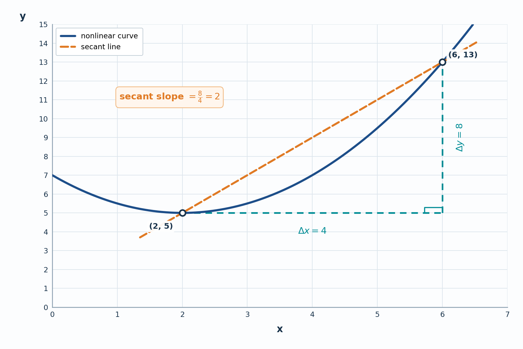
When information is shown on a graph, begin by identifying the coordinates of the two selected points. Suppose a curve passes through (2,5) and (6,13):
The average rate of change is the slope between these points:
6−213−5=48=2
The average rate is 2 vertical units per horizontal unit over the interval [2,6]. If the points do not fall exactly on grid intersections, read their coordinates as carefully as possible and report the result as an estimate.
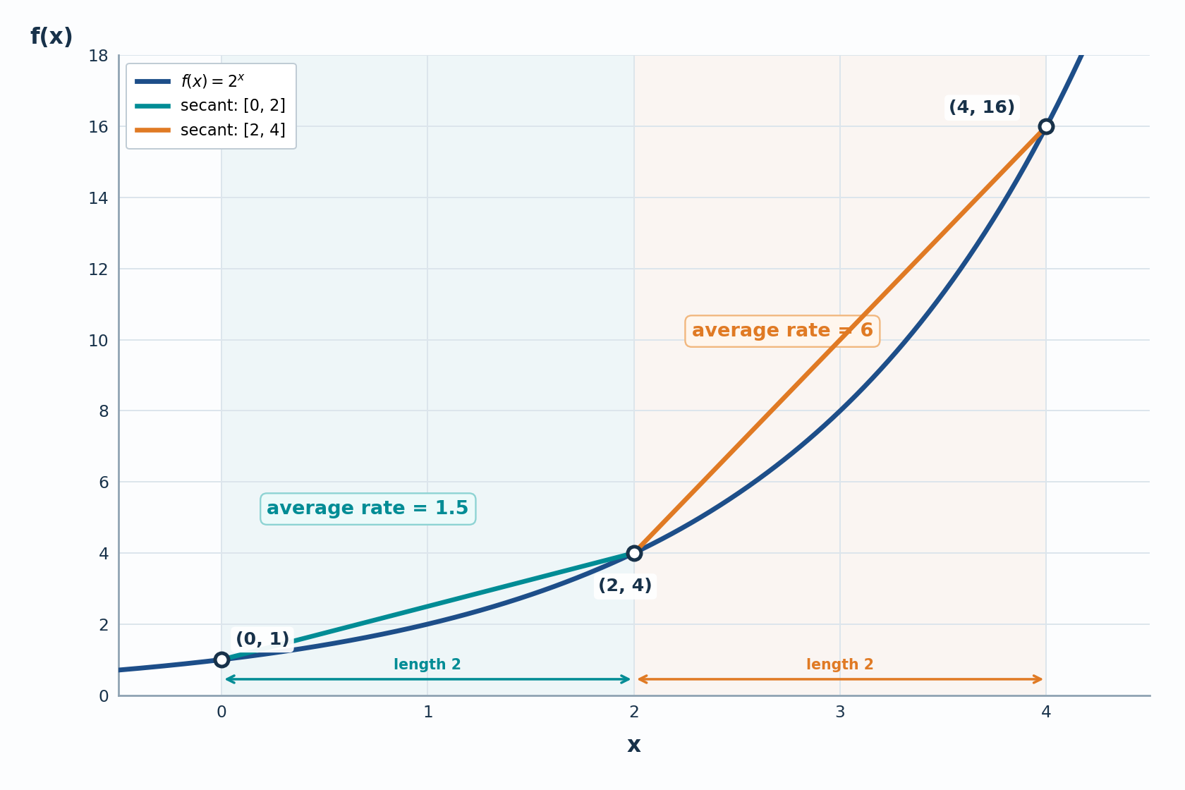
The examples above show an important feature of nonlinear functions: the same function can have different average rates on different intervals. Consider the exponential function f(x)=2x.
From x=0 to x=2:
2−0f(2)−f(0)=24−1=1.5
From x=2 to x=4:
4−2f(4)−f(2)=216−4=6
Both intervals have a length of 2 input units, but the second average rate is four times larger. This matches the shape of an exponential growth graph, which becomes steeper as x increases.
For this reason, an answer such as "the average rate is 6" is incomplete by itself. State the interval as well: the average rate is 6 on [2,4].
A numerical answer becomes more useful when you interpret its sign. The sign describes the overall change from the first endpoint to the second, not necessarily what happened at every point in between.
Sign of average rate
Endpoint relationship
Overall meaning
Positive
f(b)>f(a)
The output is higher at the end of the interval
Negative
f(b)<f(a)
The output is lower at the end of the interval
Zero
f(b)=f(a)
There is no net change between the endpoints
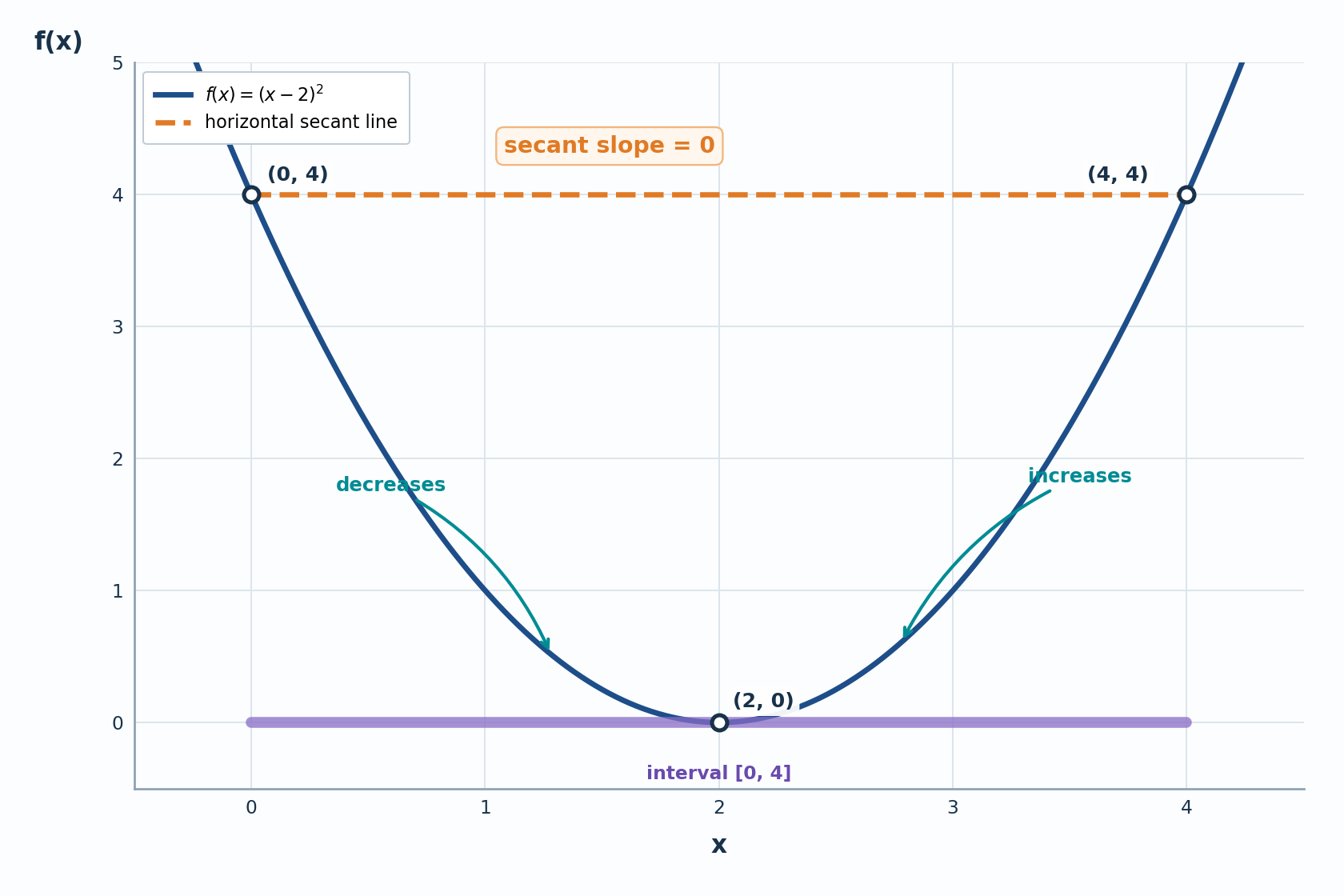
A zero average rate does not necessarily mean that the graph stayed flat. Consider f(x)=(x−2)2 on [0,4]:
f(0)=4andf(4)=4
4−0f(4)−f(0)=44−4=0
The graph decreases to a minimum and then increases, but its endpoint outputs are equal:
Units come from dividing the output units by the input units. For example, if a tank holds 80 liters at 2 minutes and 50 liters at 7 minutes, then:
7−250−80=5−30=−6 liters per minute
The negative sign means that the amount of liquid decreases by an average of 6 liters per minute.
You can use the following process for average-rate problems from equations, tables, or graphs:
Identify the interval. Label the two input endpoints a and b.
Find the endpoint outputs. Determine f(a) and f(b), either by substitution, by reading a table, or by reading coordinates from a graph.
Calculate both changes. Find the output change f(b)−f(a) and the input change b−a.
Divide and interpret. Calculate the quotient, then state its sign, units, and interval.
Writing the output change and input change separately helps you avoid mixing inputs with outputs. It also makes it easier to check whether the denominator represents the full width of the interval.
The most frequent errors are easy to prevent when you check each part of the formula:
Dividing by an endpoint such as b instead of dividing by the input change b−a.
Pairing the output from one endpoint with the input from the other endpoint.
Reporting only the total output change instead of dividing by the input change.
Treating the average rate as the exact rate at every point in a nonlinear interval.
Reversing the order in only the numerator or only the denominator.
Ignoring a negative sign or leaving out the interval and units when the context provides them.
A useful self-check is to examine the units: output units should appear in the numerator, input units should appear in the denominator, and the final answer should have units such as miles per hour, dollars per item, or liters per minute.
Average rate of change compares the change in output with the change in input, using b−af(b)−f(a). It is the slope of the secant line through two points on a graph. For nonlinear functions, the interval is part of the answer, while the sign and units explain the direction and meaning of the change.
In the practice section that follows, you will find average rates from equations, tables, and graphs. Use the four-step method to organize each calculation, then check whether your result makes sense for the interval and context.