Welcome, space explorer, to JAX in Action: Neural Networks from Scratch! This lesson marks the exciting start of our third course together. We're about to take all those fantastic JAX skills you've been honing and apply them to building neural networks, piece by piece.

Let's quickly chart our journey so far. In our first course, JAX Fundamentals: NumPy Power-Up, you became proficient with JAX's core elements, like immutable arrays, the beauty of pure functions, the magic of automatic differentiation (jax.grad), and the speed boosts from just-in-time (JIT) compilation (jax.jit). Then, in Advanced JAX: Transformations for Speed & Scale, we explored powerful functional transformations. You learned about JAX's explicit random number generation, mastered batch processing with jax.vmap, got a glimpse of multi-device parallelism with jax.shard_map, learned to handle complex data structures with PyTrees, and picked up essential profiling and debugging techniques.

Now, in this course, we'll use this powerful toolkit to construct neural networks. We'll begin with the fundamentals, like implementing Multi-Layer Perceptrons (MLPs), and progressively build more complex models, eventually leveraging JAX ecosystem libraries like Flax and Optax. In this first lesson, we'll tackle the classic XOR problem. It's a perfect way to understand non-linear classification. Our focus today will be on the crucial first steps: preparing our data and initializing the network's parameters.

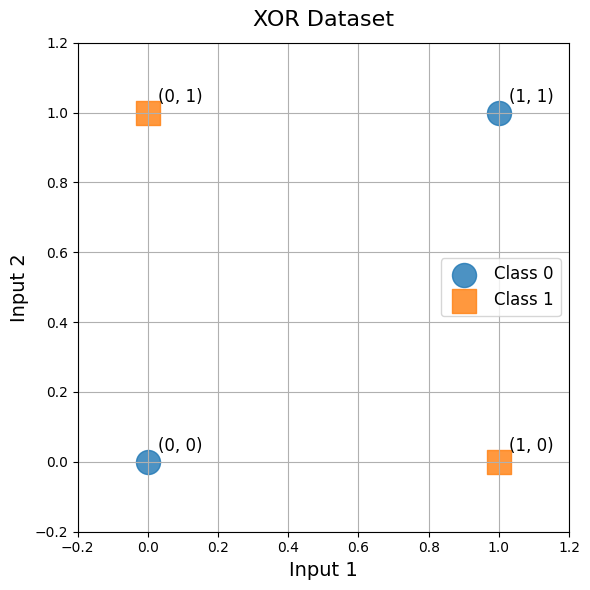
The XOR (exclusive OR) problem is a cornerstone in the study of neural networks. It's a simple yet profound example that highlights why we often need networks with multiple layers. The XOR function takes two binary inputs (0 or 1) and produces a binary output. The rule is: the output is 1 if the inputs are different and 0 if they are the same. Let's visualize this via a truth table:

If you try to plot these four points on a 2D graph, you'll notice something interesting: you can't draw a single straight line to separate the points that result in an output of 0 from those that result in an output of 1. This property is called linear inseparability. A single-layer perceptron, which can only learn linear decision boundaries, would be stumped by XOR! This is why XOR is such a great example to show the power of multi-layer networks, which can learn the necessary non-linear patterns.

First things first, let's prepare our dataset for the XOR problem using JAX arrays. It's important to structure our data correctly. The input features will be a 2D array, where each row is a distinct data point (an input pair like [0,0]), and each column represents a feature. The target labels, which are the desired outputs, will be a 2D column vector.

In this snippet, we define xor_X to hold our four input pairs and xor_y for their corresponding outputs. We've explicitly set dtype=jnp.float32. Neural networks typically perform calculations using 32-bit floating-point numbers for a good balance of precision and computational efficiency. Our input xor_X has a shape of (4, 2), meaning 4 data samples, each with 2 features. The target xor_y has a shape of (4, 1), making it a column vector. Maintaining consistent shapes like this is vital for smooth operations later on, especially during the forward and backward passes of our network.

To solve the XOR problem, we need a Multi-Layer Perceptron (MLP) with at least one hidden layer. This hidden layer is what allows the network to learn non-linear relationships. We'll design a simple yet effective architecture:

1. An input layer that matches the number of features in our data.
2. A hidden layer with a few neurons to capture the XOR logic.
3. An output layer that produces our single binary prediction.

Let's define the sizes for these layers:

This code sets up mlp_layer_sizes as [2, 3, 1]. This means our network will have:

• 2 neurons in the input layer (one for each input feature of XOR).
• 3 neurons in the hidden layer. While 2 hidden neurons are theoretically enough for XOR, using 3 gives a bit more capacity and makes our example slightly more general.
• 1 neuron in the output layer (to predict the single 0 or 1 output).

This list, mlp_layer_sizes, will be very handy when we initialize the weights and biases for our network, as it dictates their dimensions.

Initializing the weights and biases of a neural network correctly is super important for effective training. If all weights start the same, all neurons in a layer will learn the same thing. Random initialization breaks this symmetry. The scale of these initial random values also matters; if they're too large or too small, it can lead to problems like vanishing or exploding gradients during training, making it hard for the network to learn.

We'll use a popular and effective method called Xavier/Glorot initialization for our weights. This technique helps keep the signal and its gradients flowing smoothly through the network by scaling the initial weights based on the number of input and output neurons for a layer. The formula for the limit used in uniform Xavier initialization is:

Now, let's write a Python function to initialize the parameters (weights and biases) for our MLP. We'll organize these parameters as a list of dictionaries. Each dictionary in the list will represent a layer and will contain its w (weights) and b (biases). This structure is a PyTree, which JAX handles very efficiently!

This function, initialize_mlp_params, iterates through the layer_sizes list. For each connection between an input layer and an output layer (e.g., input layer to hidden layer, then hidden layer to output layer), it:

1. Splits the current_key to get new, unique keys (w_key, ) for initializing weights and biases. This is crucial for JAX's functional approach to randomness.

Let's put all the pieces together and inspect what we've created. We'll print our XOR data and the structure of our initialized MLP parameters. This helps confirm that the shapes and data types are as we expect.

When you run this code (for example, by placing the xor_X, xor_y, mlp_layer_sizes definitions and the initialize_mlp_params function before main, and then calling main()), you'll see output like this:

Look at that! Our input features X are (4, 2) and labels are , just as planned. The MLP parameters also have the correct shapes:

Fantastic job today! You've successfully laid the groundwork for building our first neural network in JAX by preparing the XOR dataset and implementing a robust parameter initialization scheme. These steps, including careful data representation and principled weight initialization like Xavier/Glorot, are fundamental to any deep learning project.

With this solid foundation in place, we're perfectly poised to bring our MLP to life in the next lesson. We'll focus on implementing the forward pass, where input data flows through the network's layers and activation functions to produce a prediction.