Recurrent Neural Networks (RNNs) are a type of neural network designed to handle sequential data, making them well-suited for time series analysis. Unlike traditional neural networks, RNNs have a unique feature called memory, which allows them to retain information from previous inputs. This ability to capture temporal dependencies is what makes RNNs powerful for tasks involving sequences, such as time series forecasting.

RNNs process data in a loop, where the output from the previous step is fed back into the network as input for the next step. This feedback loop enables RNNs to learn patterns and dependencies over time, making them ideal for analyzing time series data.

The structure of an RNN consists of a series of interconnected nodes, or neurons, organized in layers. Each neuron in the hidden layer receives input from the previous layer and passes its output to the next layer. The key feature of RNNs is the recurrent connection, where the output of a neuron is fed back into itself, allowing the network to maintain a memory of previous inputs. This structure enables RNNs to process sequences of data and learn temporal patterns.

The diagram below illustrates how this structure differs from a standard Feedforward Neural Network (FNN), highlighting the key addition of recurrent connections in RNNs.

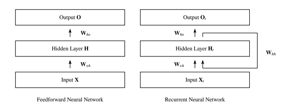
Diagram source: Robin M. Schmidt, “Recurrent Neural Networks (RNNs): A Gentle Introduction and Overview”, 2019.

In more detail, an RNN typically consists of an input layer, one or more hidden layers, and an output layer. The hidden layers are where the recurrent connections occur. At each time step, the hidden state is updated based on the current input and the previous hidden state. This update is usually performed using a non-linear activation function, such as the hyperbolic tangent (tanh) or the rectified linear unit (ReLU).

The recurrent nature of RNNs allows them to share parameters across different time steps, which makes them efficient for modeling sequences. However, this also leads to challenges such as the vanishing gradient problem, where gradients can become very small, making it difficult for the network to learn long-range dependencies. To address this, variants of RNNs like Long Short-Term Memory (LSTM) and Gated Recurrent Unit (GRU) have been developed, which include mechanisms to better capture long-term dependencies. We will discuss these methods in more detail later.

Time series data is a sequence of data points collected or recorded at specific time intervals. It is crucial in various fields, including finance, meteorology, and transportation, as it helps in understanding trends, making forecasts, and identifying patterns over time.

Time series data has unique characteristics such as trends, seasonality, and noise. A trend is a long-term increase or decrease in the data, while seasonality refers to periodic fluctuations that occur at regular intervals. Noise is the random variation in the data that cannot be attributed to any specific pattern. Real-world examples of time series data include stock prices, weather data, and the number of airline passengers over time.

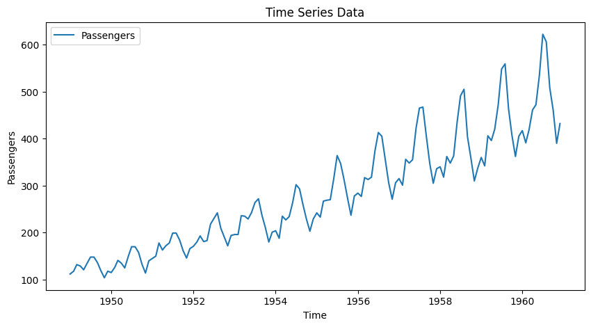
The Airline Passenger Traffic dataset is a classic example of time series data, often used to demonstrate time series analysis techniques. It contains monthly totals of international airline passengers from 1949 to 1960. This dataset is valuable for illustrating trends, seasonality, and other time series characteristics.

For convenience, we have stored this dataset in a CSV file named data.csv, which contains a Month column representing the time intervals and a Passengers column representing the number of passengers. This setup allows you to easily load and work with the dataset in your environment.

If you prefer, you can also access this dataset from various online sources, such as Kaggle or the UCI Machine Learning Repository. Additionally, it is available in some Python libraries like statsmodels as a built-in dataset. Here's how you can load the dataset using statsmodels:

This code demonstrates how to load the Airline Passenger Traffic dataset using the statsmodels library.

Before we dive into working with time series data, it's important to set up your Python environment. In this course, we will use libraries like Pandas and Matplotlib for data manipulation and visualization. If you're working on your own device, you can install these libraries using pip:

However, if you're using the CodeSignal environment, these libraries are pre-installed, so you don't need to worry about setting them up.

Let's start by loading the Airline Passenger Traffic dataset using Pandas. We'll use a dataset containing the number of airline passengers over time. First, we'll read the data from a CSV file and convert the Month column to a datetime format. Then, we'll set the Month column as the index to facilitate time-based operations.

Once the data is loaded, we'll use Matplotlib to visualize the time series. Plotting the data helps us identify patterns, trends, and any anomalies present in the dataset.

Here's the code to load and visualize the time series data:

When you run print(df.head()), the output will display the first five rows of the dataset, which might look something like this:

This output shows the Month and Passengers columns, allowing you to verify that the data has been loaded correctly.

The output of this plot is a line graph that displays the number of airline passengers over time. The x-axis represents the time in months, while the y-axis represents the number of passengers. This visualization helps in identifying trends, seasonality, and any anomalies present in the dataset.

Let's walk through the code example step-by-step. We begin by importing the necessary libraries, Pandas and Matplotlib. Pandas is used for data manipulation, while Matplotlib is used for plotting.

Next, we load the dataset using pd.read_csv('data.csv'). The dataset contains a Month column and a Passengers column. We convert the Month column to a datetime format using pd.to_datetime(df['Month']) and set it as the index with df.set_index('Month', inplace=True). This allows us to perform time-based operations on the data.

Finally, we use Matplotlib to plot the data. We create a figure with plt.figure(figsize=(10, 5)) and plot the Passengers column with plt.plot(df, label="Passengers"). We add a title, labels, and a legend to the plot for clarity. The plot is displayed using plt.show(), allowing us to visually analyze the time series data.

In this lesson, we introduced Recurrent Neural Networks (RNNs) and their ability to handle sequential data. We discussed the structure of RNNs and how they process data in a loop to learn temporal patterns. We also explored the concept of time series data and its significance in various fields, highlighting its characteristics such as trends and seasonality.

We introduced the Airline Passenger Traffic dataset, a classic example of time series data, and guided you through setting up your Python environment. We demonstrated how to load and visualize this dataset using Pandas and Matplotlib. Visualizing time series data is a crucial step in identifying patterns and trends, which lays the foundation for further analysis.

As you move on to the practice exercises, you'll have the opportunity to reinforce the concepts learned in this lesson. These exercises will help you gain hands-on experience in working with time series data and prepare you for the next unit, where we'll delve deeper into preparing time series data for RNNs.