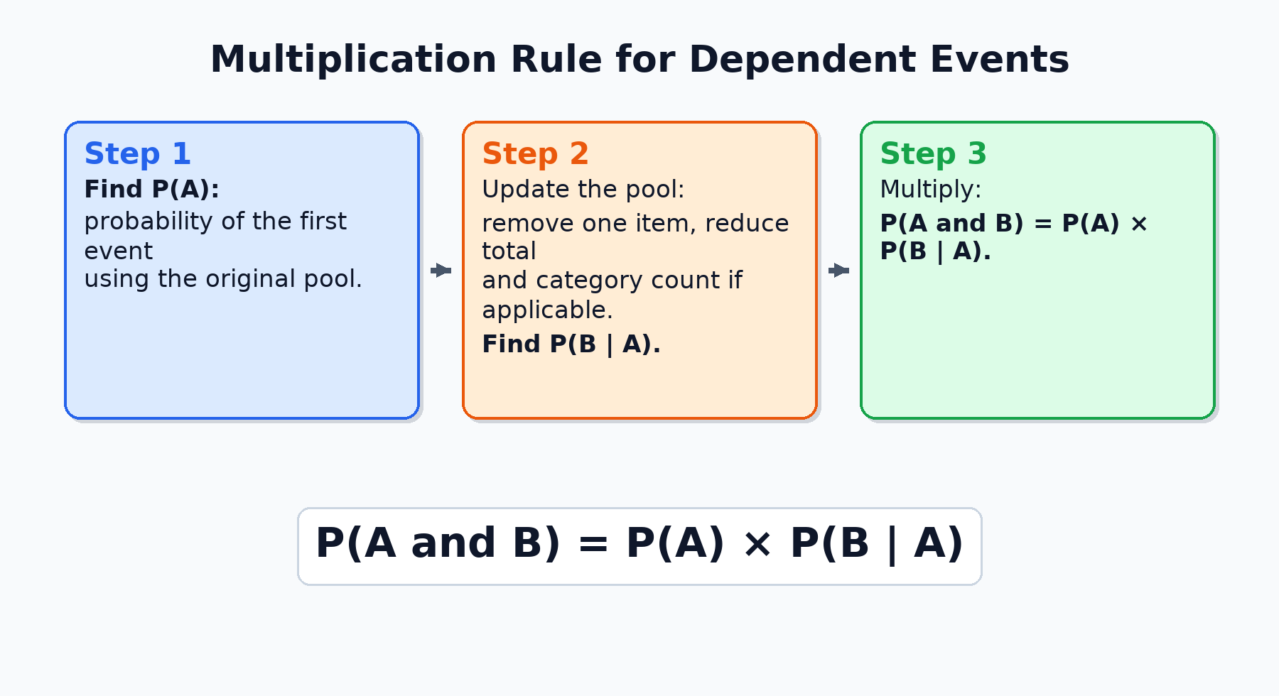
Welcome back to How Events Influence Each Other! This is Lesson 4 of 5, so we are almost at the finish line of this course. In the previous lesson, we discovered that dependent events reshape the playing field for each other: removing an item from a pool shifts both the total count and the category counts, giving the second event a different probability than it started with. We traced those shifts in detail, but we stopped short of one crucial skill — computing the overall probability that both events happen together.
That is exactly what this lesson delivers. We will give the "updated probability" a formal name, introduce a clean formula, and apply it step by step through two real-world examples. By the end, you will have a reliable three-step process you can use whenever two dependent events need to be combined.
From Observation to Calculation
Recall the employee scenario from Lesson 3: a team of 10 people (4 engineers, 6 designers) had one member randomly removed, and the probability of picking an engineer on the second draw turned out to be either 93 or 94, depending on who left first. That adjusted fraction — computed after accounting for the first event's result — has a formal name: conditional probability.
Conditional probability captures the likelihood of the second event given that the first event has already occurred and its result is known. It is the bridge between simply recognizing dependence and calculating with it. Once we pair this adjusted probability with the probability of the first event, a single multiplication will give us the combined result we are after.
The Notation: P(B | A)
Join the 1M+ learners on CodeSignal
Be a part of our community of 1M+ users who develop and demonstrate their skills on CodeSignal
Probability uses a compact shorthand for conditional probability. We write P(B∣A) and read it as "the probability of B given A." The vertical bar means "given that" or "assuming that."
This is the same updated fraction we already computed informally in Lesson 3. For example, if we want the probability of drawing a second engineer after one engineer has already been removed, we write P(second is engineer∣first is engineer) and evaluate it using the reduced pool. The important point is that P(B∣A) is generally not equal to P(B), because event A has already changed the conditions.
With this notation in hand, we can state the rule. To find the probability that two dependent events A and Bboth occur, multiply:
P(A and B)=P(A)×P(B∣A)
You might notice this looks a lot like the independent multiplication rule from Lesson 2: P(A and B)=P(A)×P(B). The only difference is that P(B) has been replaced by P(B∣A), the conditional probability that reflects the new conditions after A has occurred.
Why does multiplication still work? Think of it this way: P(A) tells us how often event A happens out of all possibilities. Then P(B∣A) tells us, among those cases where A happened, how often B also occurs. Multiplying these two fractions gives the overall share of cases where both events happen together.
Let's put the formula into action. A bag holds 5 red marbles and 3 blue marbles (8 total). We draw two marbles one after the other without replacement. What is the probability that both are red?
Step 1 — Find P(A).
Event A: the first marble is red. There are 5 red out of 8 total:
P(A)=85
Step 2 — Find P(B∣A).
Event B: the second marble is red. Because one red marble is already gone, the bag now holds 4 red and 3 blue (7 total):
P(B∣A)=74
Step 3 — Multiply.
P(A and B)=85×74=5620=145≈0.357
The probability of drawing two red marbles in a row is about 35.7%. Notice how both the numerator (from 5 to 4) and the denominator (from 8 to 7) decreased for the second fraction. Tracking both of these changes is the core skill in every dependent-probability problem.
Now let's apply the same three steps in a workplace setting. A bin at a warehouse contains 10 items: 4 are defective and 6 function properly. A worker randomly pulls two items in a row without returning the first. What is the probability that both items are defective?
Step 1 — Find P(A).
P(A)=104=52
Step 2 — Find P(B∣A).
After removing one defective item, the bin holds 3 defective and 6 working items (9 total):
P(B∣A)=93=31
Step 3 — Multiply.
P(A and B)=52×31=152≈0.133
There is roughly a 13.3% chance that both pulled items are defective. The pattern is identical to the marble example: one item leaves the pool, the total drops by one, and the count of the target category also drops by one because the first item drawn belonged to that category.
In the previous examples, we looked for two items of the same type (two red marbles or two defective parts). However, the multiplication rule works exactly the same way when the events involve different categories. The core logic—updating the pool before the second calculation—remains your north star.
Imagine a bag with 4 red, 3 green, and 3 blue marbles (10 total). What is the probability of drawing a red marble first and a green marble second without replacement?
Step 1 — Find P(Red).
There are 4 red marbles out of 10.
P(A)=104
Step 2 — Find P(Green∣Red).
After removing one red marble, the bag now contains 3 red, 3 green, and 3 blue items. The total has dropped to 9. Crucially, since the first marble was red, the number of green marbles is still 3.
P(B∣A)=93
Step 3 — Multiply.P(A and B)=104×93=9012=152≈0.133
Even though the categories changed, the process didn't. We still updated the total (the denominator) because an item was removed, and we updated the specific category count (the numerator) based on what exactly was removed.
As you start applying this rule on your own, watch out for these frequent pitfalls:
Forgetting to reduce the denominator. After one item is removed, the total shrinks by one. Using the original total in the second fraction is the single most common error.
Forgetting to adjust the numerator. If the first item belonged to the category you care about (e.g., red, defective), the favorable count drops by one as well. If the first item came from a different category, the favorable count stays the same — only the denominator changes.
Using the independent rule by habit. Writing P(A)×P(B) instead of P(A)×P(B∣A) ignores the changed conditions and produces an incorrect answer.
A helpful habit: right after writing P(A), pause and ask yourself, "What is left in the pool now?" Update both the total and the category count before writing the second fraction. This small pause will prevent the vast majority of errors.
When two events are dependent, we calculate the probability that both occur using P(A and B)=P(A)×P(B∣A). The key is computing P(B∣A) — the conditional probability that reflects the updated pool after the first event. This means adjusting both the numerator and the denominator to match what remains, then multiplying. Whether the scenario involves marbles, warehouse bins, or any other shrinking pool, the three-step process is always the same: find P(A), update the pool, find P(B∣A), and multiply.
Now it is your turn to put the formula to work. The practice tasks ahead will walk you through card decks, team rosters, sock drawers, and quality inspections — giving you plenty of chances to make the three-step process second nature.