In the first lesson of Horizontal Shifts: Sliding Left and Right, we settled the why: a constant inside f acts on the input, and the graph travels the opposite way from what the sign appears to suggest. This is the second of three lessons, so we are right in the middle of the course, and the question now turns from why to how.
Knowing the direction is only half a skill. In this lesson we will turn that rule into a routine we can carry out quickly and confidently: take any parent graph, slide it sideways on purpose, produce the shifted table of values, and state exactly where its most important points land.
One Rule, Written as a Point Map
Everything in this lesson comes from a single line. If g(x)=f(x−h), then each point (x,y) on the graph of f moves to
(x,y)⟶(x+h,y)
Notice what changes and what does not: the first coordinate gains h, and the second coordinate is copied over untouched. This is the mirror image of the vertical rule (x,y)→(x,y+k) from the previous course, where the output moved and the input stayed put.
It is also worth noticing that the point map contains no minus sign at all, even though the formula does. The reversal was already absorbed the moment we wrote the shift in the standard form f(x−h), which is exactly why that form is worth insisting on.
Moving a Handful of Points
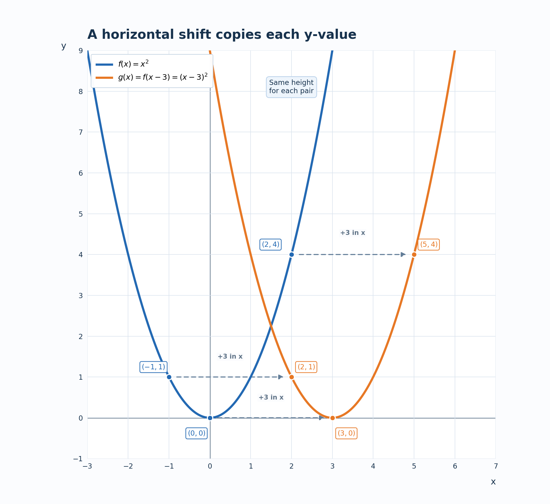
Let us try the map on f(x)=x2 with g(x)=f(x−3). Here h=3, so every point travels three units right, and all we do is add 3 to each x-coordinate.
Point on f
Shifted point on g
(−1,1)
(2,1)
(0,0)
(3,0)
(2,4)
(5,4)
Each tracked point slides horizontally while keeping exactly the same height.
A quick spot-check keeps us honest on the middle row: g(3)=f(3−3)=f(0)=0, which matches. A negative h behaves no differently. For g(x)=f(x+3) we rewrite the inside as f(x−(−3)), so h=−3, each x-coordinate loses three, and (2,4) lands at (−1,4).
Join the 1M+ learners on CodeSignal
Be a part of our community of 1M+ users who develop and demonstrate their skills on CodeSignal
Tables make the idea especially vivid, because we never recompute a single output. We keep the output column exactly as it stands and only relabel the inputs that produce it. Continuing with f(x)=x2 and g(x)=f(x−3):
x for f
x for g
shared output
−2
1
4
−1
2
1
0
3
0
1
4
1
2
5
4
The output column still reads 4,1,0,1,4, in that same order. A horizontal shift relocates outputs; it never changes them. So if a shifted table shows different y-values than the original, that is a reliable signal that something went wrong.
As you may recall from the first course, each parent graph has an anchor point that we track before anything else. Under a horizontal shift the anchor obeys the same map, and the rest of the curve follows along:
y=x2, vertex (0,0): under f(x−4) it becomes (4,0).
y=∣x∣, corner (0,0): under f(x+5), so h=−5, it becomes (−5,0).
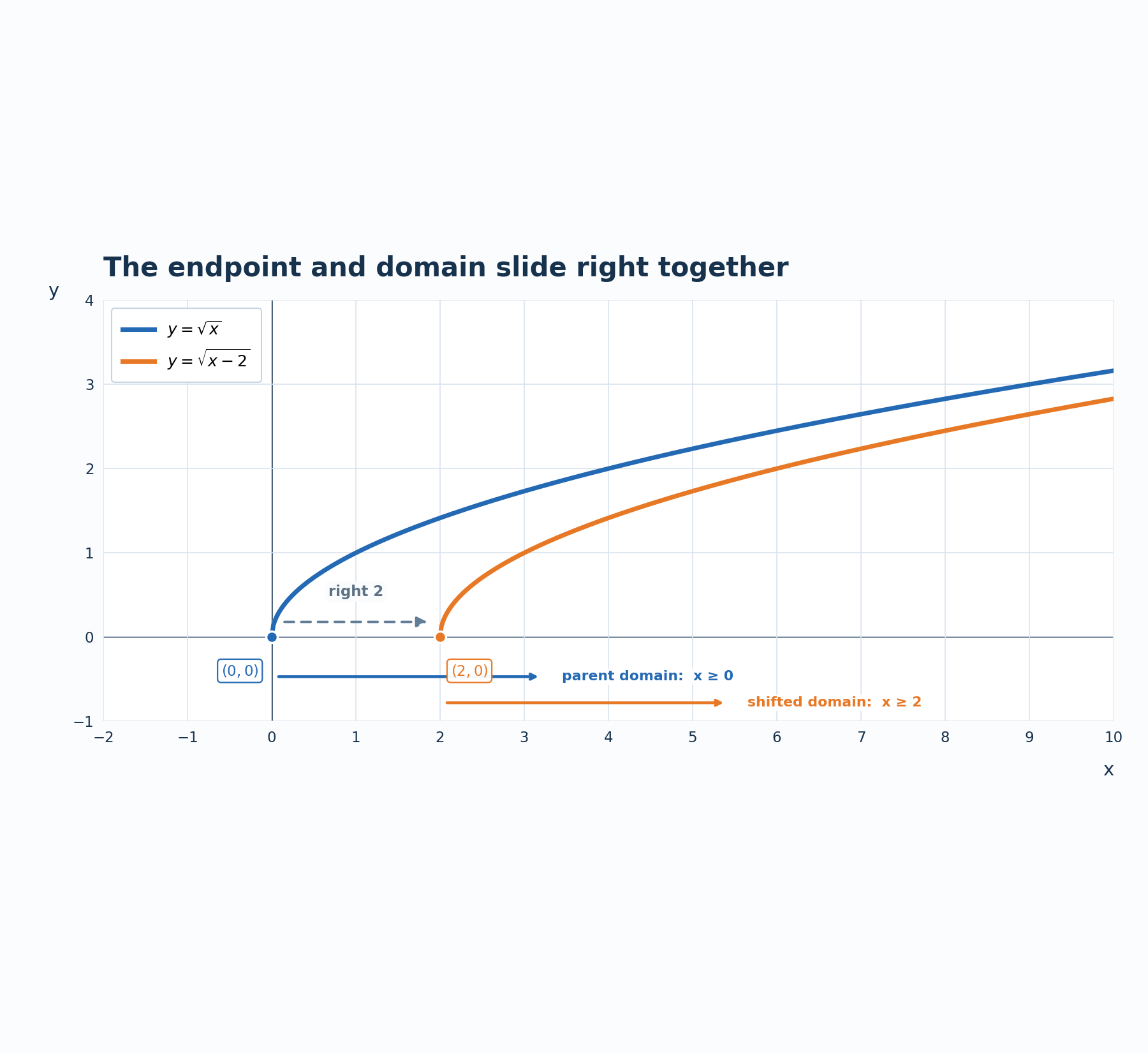
y=x, endpoint (0,0): under f(x−2) it becomes (2,0), and the domain becomes x≥2.
The square-root case deserves a second look, since that graph starts at its endpoint and exists only to the right of it. Sliding it right by 2 carries the entire domain along with it.
x-intercepts are just as obedient: if f(x)=x2−9 crosses at x=−3 and x=3, then f(x−2) crosses at x=−1 and x=5. The y-intercept is the one feature we cannot simply slide, because the y-axis refuses to move with the graph; instead we evaluate directly, so here g(0)=f(0−2)=f(−2)=−5.
With those features in hand, a clean sketch of f(x−h) takes only three moves.
Read the signed h from the standard form f(x−h), so f(x+7) gives h=−7.
Move the anchor point (or endpoint) by adding h to its x-coordinate.
Move two or three nearby reference points the same way, then redraw the familiar shape through them.
The shape itself never needs rethinking. A horizontal shift is a rigid translation: no stretching, no flipping, no change in steepness or width, just the same curve parked in a new place.
Time-based situations give this rule an everyday meaning. Suppose v(t) is the number of viewers of a livestream t minutes after it begins, and one week the host starts the stream 10 minutes late. At clock time t the stream has been running for only t−10 minutes, so the new viewer count is v(t−10), with h=10 and a graph shifted right.
The practical reading is that every milestone happens later by the same amount, while the milestone values stay identical. If the peak audience of 500 used to occur at t=25, it now occurs at t=35, and it is still exactly 500 people.
A head start reverses the story. The function v(t+10) describes a stream that began ten minutes early, so at any clock time the audience is already further into the broadcast, every event arrives sooner, and the curve slides left.
We now have a complete working method for f(x−h). Read the signed h, apply (x,y)→(x+h,y) to the anchor and a few reference points, copy the output column of any table without touching it, and remember that endpoints and x-intercepts travel while the y-intercept must be recomputed. In a timing context, a positive h is a delay and a negative h is a head start.
Time to make it yours. The exercises ahead will have us sliding anchors of several parent graphs, filling in shifted tables, tracking endpoints and intercepts on a plot, telling horizontal shifts apart from vertical ones using raw numbers alone, and rescuing a store sale that starts two days behind schedule.