Welcome to the first lesson of the course "Handling Multivariate Time Series with RNNs." In this lesson, we will lay the groundwork for understanding and preprocessing multivariate time series data. A multivariate time series consists of multiple variables recorded over time, which is crucial for forecasting as it considers interactions between different variables for more accurate predictions.

We will be working with the Air Quality dataset from the UCI Machine Learning Repository, accessible here. This dataset contains 9358 instances of hourly averaged responses from a gas multisensor device deployed in an Italian city. It includes 15 features, such as concentrations of air pollutants (e.g., CO, NOx, C6H6) and meteorological data (e.g., temperature, humidity). The data was recorded from March 2004 to February 2005. The dataset uses -200 to represent missing values, which we will replace with NaN during preprocessing to ensure accurate data handling. Our goal is to perform multivariate time series analysis, which involves handling missing values to ensure accurate modeling and predictions.

To begin, we need to load the Air Quality dataset into our environment. We will use the pandas library, which is a powerful tool for data manipulation and analysis in Python. The dataset is hosted on an AWS S3 URL, and we can load it directly from there. It's important to handle missing values during the loading process to ensure the integrity of our data.

Here's how you can load the dataset:

In this code, we use pd.read_csv() to read the CSV file from the specified URL. The sep=';' parameter indicates that the data is separated by semicolons, and decimal=',' specifies that commas are used as decimal points. We also replace -200 with NaN to correctly identify missing values. This step is crucial for correctly interpreting the numerical data.

The dataset contains separate Date and Time columns, which we need to combine into a single DateTime column. This combination is essential for time series analysis, as it allows us to work with a unified time index.

Here's how you can combine these columns:

In this example, we use pd.to_datetime() to convert the combined Date and Time strings into a datetime object. The format parameter specifies the format of the input strings, ensuring accurate conversion.

Cleaning the dataset involves removing unnecessary columns and handling missing values. This step is vital to ensure that our data is ready for analysis and modeling.

First, we drop the original Date and Time columns, as they are no longer needed:

Next, we remove any columns that are not essential for our analysis:

We also need to address missing values. For essential features, we drop rows where these values are missing:

For other missing values, we use forward-fill and backward-fill techniques to fill them. Forward-fill is applied first to propagate the last valid observation forward to the next valid observation, which is useful when the previous value is a reasonable estimate for the missing data. After forward-filling, backward-fill is used to fill any remaining gaps by propagating the next valid observation backward, ensuring that all missing values are addressed comprehensively. This two-step approach helps maintain the continuity and integrity of the time series data.

These steps ensure that our dataset is clean and complete, ready for further analysis.

Setting the DateTime column as the index is crucial for time series analysis. It allows us to perform operations that are specific to time series data, such as resampling and rolling statistics.

Here's how you can set the DateTime column as the index:

By setting the DateTime column as the index, we can now leverage pandas' time series functionality to analyze and manipulate our data effectively.

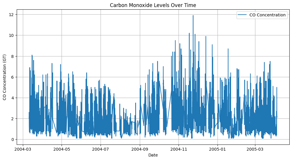
Visualizing the data is an important step to understand the trends and patterns in the time series. We will use the matplotlib library to create a simple line plot of one of the features, such as CO(GT).

Here's how you can create a visualization:

This code generates a line plot of the CO(GT) feature over time, enabling us to visually examine the data for trends, patterns, or anomalies. By analyzing the plot, we can gain insights into the behavior of the CO(GT) levels throughout the recorded period. Additionally, you can substitute CO(GT) with any other feature from the dataset to explore and visualize different aspects of the data, providing a comprehensive understanding of the multivariate time series. The output will provide a clear visual representation of the selected feature's temporal dynamics, as shown below.

After preprocessing, it's important to verify that our dataset is clean and ready for analysis. We can display the first few rows of the cleaned dataset to ensure that all steps have been executed correctly.

This command will output the first few rows of the dataset, allowing us to visually inspect the results of our preprocessing steps.

In this lesson, we covered the essential steps for understanding and preprocessing multivariate time series data. We loaded the Air Quality dataset, replaced -200 with NaN, combined date and time columns, cleaned the dataset by removing unnecessary columns and handling missing values, set the DateTime column as the index, and visualized the data. These steps are crucial for preparing the data for further analysis and modeling.

As you move on to the practice exercises, you'll have the opportunity to reinforce these concepts and gain hands-on experience with the preprocessing techniques covered in this lesson. Remember, proper preprocessing is key to ensuring accurate time series forecasting.