Welcome to the final lesson in your journey of handling multivariate time series with Recurrent Neural Networks (RNNs). In the previous lesson, you learned how to build and train an RNN model to predict Temperature (T) using multiple features from the Air Quality dataset. Now, we will focus on evaluating the performance of this RNN model. Evaluating model performance is crucial as it helps you understand how well your model is making predictions and where improvements can be made. In this lesson, we will use the Root Mean Squared Error (RMSE) as our key evaluation metric. RMSE is widely used in regression tasks as it provides a measure of the differences between predicted and actual values.

Before we dive into evaluating the model, let's quickly recap the steps we took to build and train the RNN model:

To visualize the training loss, you need to access the history object, which is returned by the model.fit() method. This History object contains the training loss and other metrics recorded during training. The history attribute of this object is a dictionary that includes the loss values for each epoch. You can use these values to plot the training loss curve:

In this plot, you can see how the training loss decreases over the epochs, indicating the model's learning progress.

To evaluate the RNN model, we first need to make predictions on the test data. This involves using the trained model to predict the target variable, Temperature (T), based on the input features. It's important to ensure that the data used for predictions has undergone the same preprocessing steps as the training data. This includes scaling the data using the same scaler that was fitted on the training data. Once the data is prepared, you can use the predict method of the model to generate predictions.

In this code, X_test represents the input data for which predictions are to be made. The predict method returns the predicted values, which are currently in the scaled form.

The predictions generated by the model are in the scaled form, as the input data was normalized during preprocessing. To evaluate the model's performance meaningfully, we need to rescale these predictions back to their original values. This is done using the inverse_transform method of the scaler. Rescaling ensures that the predicted values are on the same scale as the actual values, allowing for accurate comparison.

In this code, the inverse_transform method is used to rescale the predicted and actual values. The np.column_stack function is used to ensure that the data has the correct shape for the inverse transformation. The rescaled predictions and actual values are now ready for evaluation.

With the predictions rescaled to their original values, we can now calculate the RMSE to evaluate the model's performance. RMSE is a measure of the average magnitude of the errors between predicted and actual values. It is calculated as the square root of the mean squared error.

In this code, the mean_squared_error function from the sklearn.metrics module is used to calculate the mean squared error between the actual and predicted values. The square root of this value gives the RMSE. A lower RMSE indicates better model performance, as it signifies smaller differences between predicted and actual values.

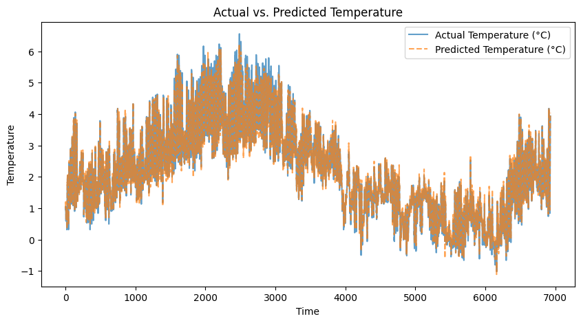
Visualization is a powerful tool for understanding model performance. By plotting the actual and predicted values, you can visually assess how well the model is capturing the patterns in the data. This can also help identify any areas where the model may be underperforming.

In this code, the matplotlib.pyplot module is used to create a plot of the actual and predicted values. The plot function is used to plot the rescaled actual and predicted values, with the predicted values displayed as a dashed line for clarity. The plot provides a visual representation of the model's performance, allowing you to see how closely the predicted values align with the actual values over time. You can see the plot output here, which shows how well the predicted values align with the actual ones overall.

In this lesson, you learned how to evaluate the performance of an RNN model for multivariate time series forecasting. We covered making predictions, rescaling them to their original values, calculating RMSE, and visualizing the results. These steps are essential for assessing how well your model is performing and identifying areas for improvement. As you move on to the practice exercises, I encourage you to apply these concepts and experiment with different parameters to deepen your understanding. Congratulations on reaching the end of the course! Your dedication and hard work have equipped you with the skills to handle multivariate time series with RNNs. Keep exploring and applying these techniques in your projects, and continue your journey in the exciting field of machine learning.