Introduction to Evaluating RNN Performance

Welcome to the final lesson in your journey of handling multivariate time series with Recurrent Neural Networks (RNNs). In the previous lesson, you learned how to build and train an RNN model to predict Temperature (T) using multiple features from the Air Quality dataset. Now, we will focus on evaluating the performance of this RNN model. Evaluating model performance is crucial as it helps you understand how well your model is making predictions and where improvements can be made. In this lesson, we will use the Root Mean Squared Error (RMSE) as our key evaluation metric. RMSE is widely used in regression tasks as it provides a measure of the differences between predicted and actual values.

Recap of Building and Training the RNN Model

Before we dive into evaluating the model, let's quickly recap the steps we took to build and train the RNN model using PyTorch, now including a train/test split for proper evaluation:

import pandas as pd
import numpy as np
from sklearn.preprocessing import StandardScaler
import torch
import torch.nn as nn
import torch.optim as optim
from torch.utils.data import DataLoader, TensorDataset

# Load the Air Quality dataset from the URL
url = "https://codesignal-staging-assets.s3.amazonaws.com/uploads/1742293523899/AirQualityUCI.csv"
df = pd.read_csv(url, sep=';', decimal=',')

# Replace -200 with NaN
df.replace(-200, np.nan, inplace=True)

# Combine 'Date' and 'Time' into a single 'DateTime' column
df['DateTime'] = pd.to_datetime(df['Date'] + ' ' + df['Time'], format="%d/%m/%Y %H.%M.%S")

# Drop the original 'Date' and 'Time' columns
df.drop(columns=['Date', 'Time'], inplace=True)

# Drop unnecessary columns
df.drop(columns=['Unnamed: 15', 'Unnamed: 16'], inplace=True)

# Drop rows where essential features are missing
df.dropna(subset=['CO(GT)', 'NO2(GT)', 'T', 'RH'], inplace=True)

# Fill missing values using forward-fill & backward-fill
df.ffill(inplace=True)
df.bfill(inplace=True)

# Set DateTime as index
df.set_index('DateTime', inplace=True)

# Select relevant features for RNN
features = ['CO(GT)', 'NO2(GT)', 'PT08.S5(O3)', 'RH', 'T']
df_selected = df[features]

# Normalize the data
scaler = StandardScaler()
df_scaled = scaler.fit_transform(df_selected)

# Function to create sequences for multi-input RNN
def create_multivariate_sequences(data, seq_length=10):
    X, y = [], []
    for i in range(len(data) - seq_length):
        X.append(data[i:i+seq_length])  # Multi-feature input
        y.append(data[i+seq_length, -1])  # Predicting Temperature (T)
    return np.array(X), np.array(y)

# Define sequence length
sequence_length = 10

# Create sequences
X, y = create_multivariate_sequences(df_scaled, sequence_length)

# Define train/test split ratio
train_ratio = 0.8
train_size = int(len(X) * train_ratio)

# Split the data
X_train, X_test = X[:train_size], X[train_size:]
y_train, y_test = y[:train_size], y[train_size:]

# Convert to PyTorch tensors
X_train_tensor = torch.tensor(X_train, dtype=torch.float32)
y_train_tensor = torch.tensor(y_train, dtype=torch.float32)
X_test_tensor = torch.tensor(X_test, dtype=torch.float32)
y_test_tensor = torch.tensor(y_test, dtype=torch.float32)

# Create DataLoader for training
train_dataset = TensorDataset(X_train_tensor, y_train_tensor)
train_dataloader = DataLoader(train_dataset, batch_size=16, shuffle=True)

# Define a modified RNN model for multivariate time series
class RNNModel(nn.Module):
    def __init__(self, input_size, hidden_size, output_size):
        super(RNNModel, self).__init__()
        self.rnn = nn.RNN(input_size, hidden_size, batch_first=True)
        self.fc1 = nn.Linear(hidden_size, 10)
        self.fc2 = nn.Linear(10, output_size)

    def forward(self, x):
        out, _ = self.rnn(x)
        out = torch.relu(self.fc1(out[:, -1, :]))
        out = self.fc2(out)
        return out

# Initialize model, loss function, and optimizer
model = RNNModel(input_size=len(features), hidden_size=30, output_size=1)
criterion = nn.MSELoss()
optimizer = optim.Adam(model.parameters(), lr=0.001)

# Train model
for epoch in range(5):
    for batch_X, batch_y in train_dataloader:
        optimizer.zero_grad()
        outputs = model(batch_X)
        loss = criterion(outputs, batch_y.unsqueeze(1))
        loss.backward()
        optimizer.step()
    print(f'Epoch [{epoch+1}/5], Loss: {loss.item():.4f}')
Plotting the Training Loss

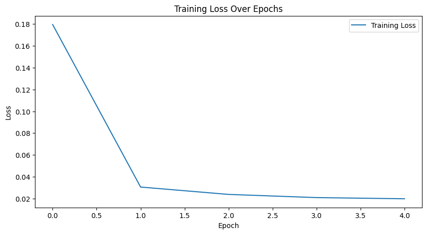
To visualize the training loss, you need to record the loss values during training and plot them using matplotlib. This helps in understanding the model's learning progress over epochs.

import matplotlib.pyplot as plt

# Assuming loss values are stored in a list called `loss_values`
loss_values = []

# Train model and record loss
for epoch in range(5):
    epoch_loss = 0
    for batch_X, batch_y in train_dataloader:
        optimizer.zero_grad()
        outputs = model(batch_X)
        loss = criterion(outputs, batch_y.unsqueeze(1))
        loss.backward()
        optimizer.step()
        epoch_loss += loss.item()
    loss_values.append(epoch_loss / len(train_dataloader))
    print(f'Epoch [{epoch+1}/5], Loss: {epoch_loss / len(train_dataloader):.4f}')

# Plot training loss
plt.figure(figsize=(10, 5))
plt.plot(loss_values, label='Training Loss')
plt.xlabel('Epoch')
plt.ylabel('Loss')
plt.title('Training Loss Over Epochs')
plt.legend()
plt.show()

In this plot, you can see how the training loss decreases over the epochs, indicating the model's learning progress.

Making Predictions with the RNN Model

To evaluate the RNN model, we first need to make predictions on the test data. This involves using the trained model to predict the target variable, Temperature (T), based on the input features. It's important to ensure that the data used for predictions has undergone the same preprocessing steps as the training data.

# Make predictions on test data
model.eval()  # Set the model to evaluation mode
with torch.no_grad():
    y_test_pred = model(X_test_tensor).squeeze().numpy()
Rescaling Predictions to Original Values

The predictions generated by the model are in the scaled form, as the input data was normalized during preprocessing. To evaluate the model's performance meaningfully, we need to rescale these predictions back to their original values.

# Rescale predictions back to original values
y_test_pred_rescaled = scaler.inverse_transform(
    np.column_stack((y_test_pred, np.zeros((len(y_test_pred), len(features) - 1)))))[:, 0]

y_test_actual_rescaled = scaler.inverse_transform(
    np.column_stack((y_test, np.zeros((len(y_test), len(features) - 1)))))[:, 0]
Calculating RMSE for Model Evaluation

With the predictions rescaled to their original values, we can now calculate the RMSE to evaluate the model's performance.

from sklearn.metrics import mean_squared_error

# Compute RMSE
rmse = np.sqrt(mean_squared_error(y_test_actual_rescaled, y_test_pred_rescaled))
print(f"RMSE: {rmse}")
Visualizing Actual vs. Predicted Values

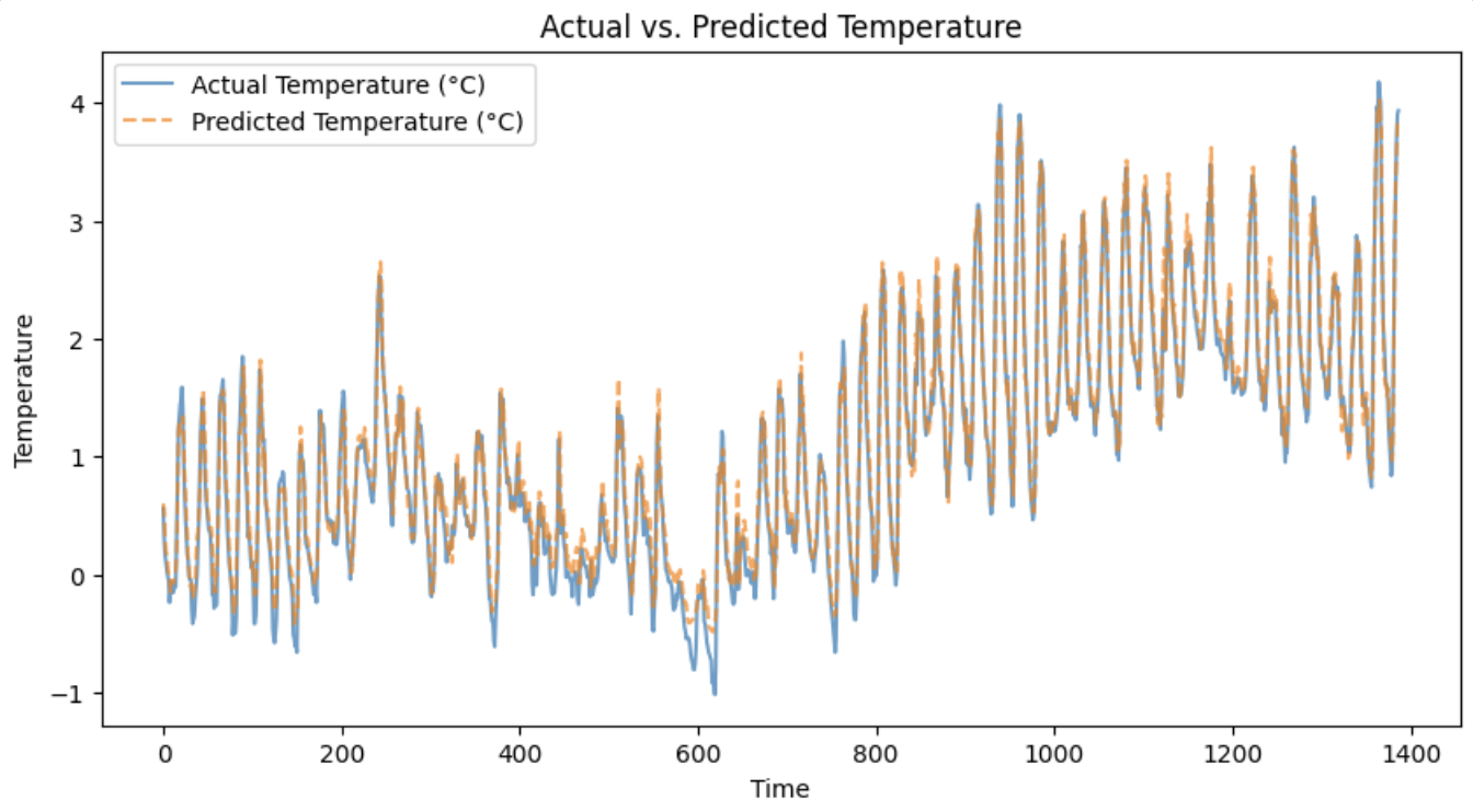
Visualization is a powerful tool for understanding model performance. By plotting the actual and predicted values, you can visually assess how well the model is capturing the patterns in the data.

# Plot actual vs. predicted values with alpha for better visibility
plt.figure(figsize=(10, 5))
plt.plot(y_test_actual_rescaled, label="Actual Temperature (°C)", alpha=0.7)
plt.plot(y_test_pred_rescaled, label="Predicted Temperature (°C)", linestyle='dashed', alpha=0.7)
plt.xlabel("Time")
plt.ylabel("Temperature")
plt.title("Actual vs. Predicted Temperature")
plt.legend()
plt.show()

You can see the plot output here, which shows how well the predicted values align with the actual ones overall.

Summary and Preparation for Practice

In this lesson, you learned how to evaluate the performance of an RNN model for multivariate time series forecasting using PyTorch. We covered splitting the data into training and test sets, making predictions, rescaling them to their original values, calculating RMSE, and visualizing the results. These steps are essential for assessing how well your model is performing and identifying areas for improvement. As you move on to the practice exercises, I encourage you to apply these concepts and experiment with different parameters to deepen your understanding.

Sign up
Join the 1M+ learners on CodeSignal
Be a part of our community of 1M+ users who develop and demonstrate their skills on CodeSignal