Estimating Pi with Darts

Estimating Pi with Darts | CodeSignal Learn

Introduction

Welcome back to Extra Tools and Practices! You have reached lesson four of four, which means this is the final stop in the entire probability learning path. That is quite an achievement, so take a moment to appreciate how far you have come. In this course alone, we modeled everyday chance scenarios, tested games for hidden bias, and used expected value to make smarter decisions. Today we close with something a little different and a lot of fun: using random dart throws to estimate the value of π . It may sound surprising that tossing darts at random could reveal one of the most famous numbers in mathematics. But as we will see, the connection between randomness and geometry runs deep, and the tools you have already learned are exactly what make it work.

The Big Idea: Randomness Meets Geometry

\pi

Setting Up the Dartboard

1 \times 1 = 1

Connecting Area to Probability

P(\text{dart inside quarter-circle}) = \frac{\text{Area of quarter-circle}}{\text{Area of square}} = \frac{\pi/4}{1} = \frac{\pi}{4}

From Probability to a π Estimate

\frac{\pi}{4}

Why More Darts Mean Better Estimates

\pi \approx 3.14159

From Random Points to Pi: The Complete Process

(x, y)

Beyond Pi: Monte Carlo in the Real World

\pi

Conclusion and Next Steps

\frac{\pi}{4}

Previous Lesson

Join the 1M+ learners on CodeSignal

Be a part of our community of 1M+ users who develop and demonstrate their skills on CodeSignal

Throughout this course, we have used probability to predict outcomes, detect fairness, and guide choices. In every case, the logic was the same: the more we know about how likely different outcomes are, the better we can reason about real situations.

Today we flip that logic around. Instead of starting with a known probability, we will run a random experiment and observe what fraction of trials meet a condition. That observed fraction approximates the theoretical probability, and from it we can back out a number we care about — in this case, $\pi$ . This approach of using repeated random trials to estimate a quantity is sometimes called a Monte Carlo method, named after the famous casino city, because it relies on chance.

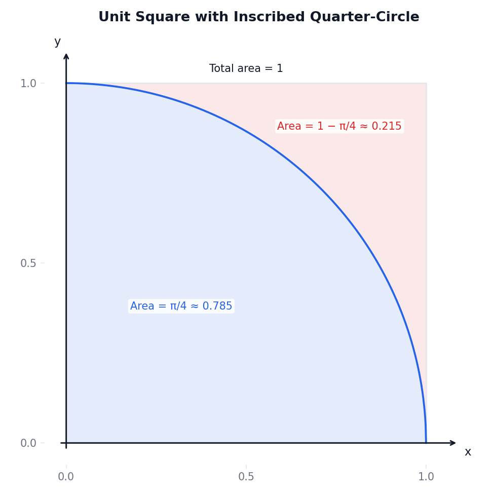
Picture a square dartboard that is 1 unit wide and 1 unit tall, with its corner at the origin of a coordinate grid. Now draw a quarter-circle of radius 1 centered at that same corner. The arc curves from the top-left corner of the square down to the bottom-right corner, and every point inside the arc is also inside the square.

Here are the two regions we care about:

The square has side length 1, so its area is $1 \times 1 = 1$ .
The quarter-circle has radius 1. A full circle of radius 1 has area $\pi r^2 = \pi$ , so one quarter of that circle has area $\frac{\pi}{4}$ .

Because the quarter-circle sits entirely inside the square, any random dart that lands in the square either lands inside the quarter-circle or outside it (but still inside the square).

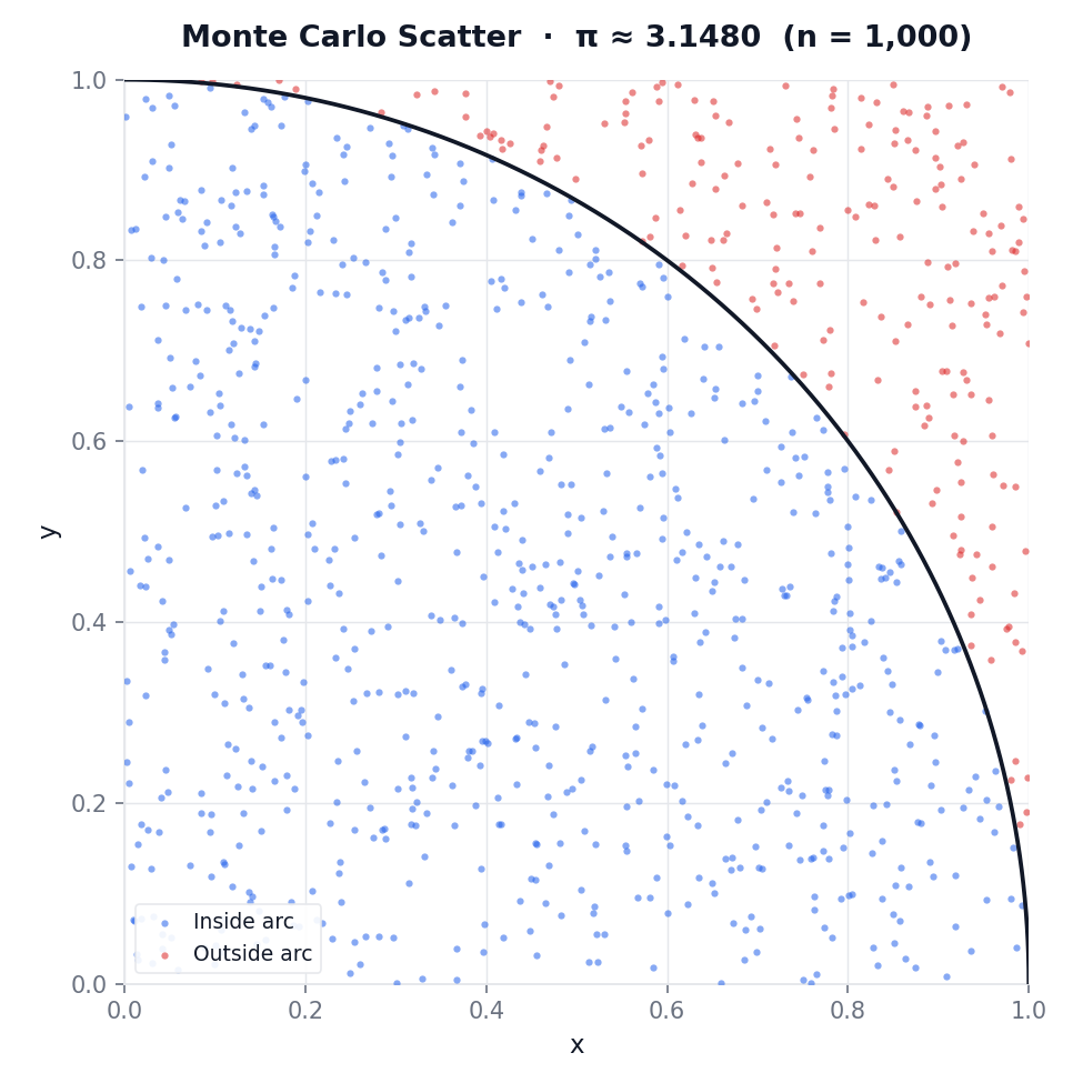
Coordinate diagram of a unit square with an inscribed quarter-circle, showing labeled area regions

Now suppose we throw a dart at the square completely at random, meaning every point inside the square is equally likely to be hit. As you may recall from earlier lessons, when outcomes are equally likely, probability equals the ratio of favorable outcomes to total outcomes. For continuous regions, "outcomes" become areas:

P(\text{dart inside quarter-circle}) = \frac{\text{Area of quarter-circle}}{\text{Area of square}} = \frac{\pi/4}{1} = \frac{\pi}{4}

So the theoretical probability of a single random dart landing inside the quarter-circle is $\frac{\pi}{4}$ , which is roughly 0.7854. This one equation is the heart of the entire method. It tells us that the fraction of darts landing inside the quarter-circle is directly linked to $\pi$ .

Conceptual illustration of darts landing inside and outside a quarter-circle inscribed in a square

If we throw a large number of darts and count how many land inside the quarter-circle, the observed proportion should be close to $\frac{\pi}{4}$ . We can rearrange that relationship to solve for $\pi$ :

\pi \approx 4 \times \frac{\text{darts inside quarter-circle}}{\text{total darts}}

Let's walk through a small example. Suppose we throw 20 darts at the unit square and 16 of them land inside the quarter-circle. Our estimate would be:

\pi \approx 4 \times \frac{16}{20} = 4 \times 0.80 = 3.20

The true value of $\pi$ is approximately 3.14159, so our estimate of 3.20 is in the right neighborhood but not very precise. That is expected with only 20 darts — a handful of lucky or unlucky throws can easily push the proportion away from the theoretical value.

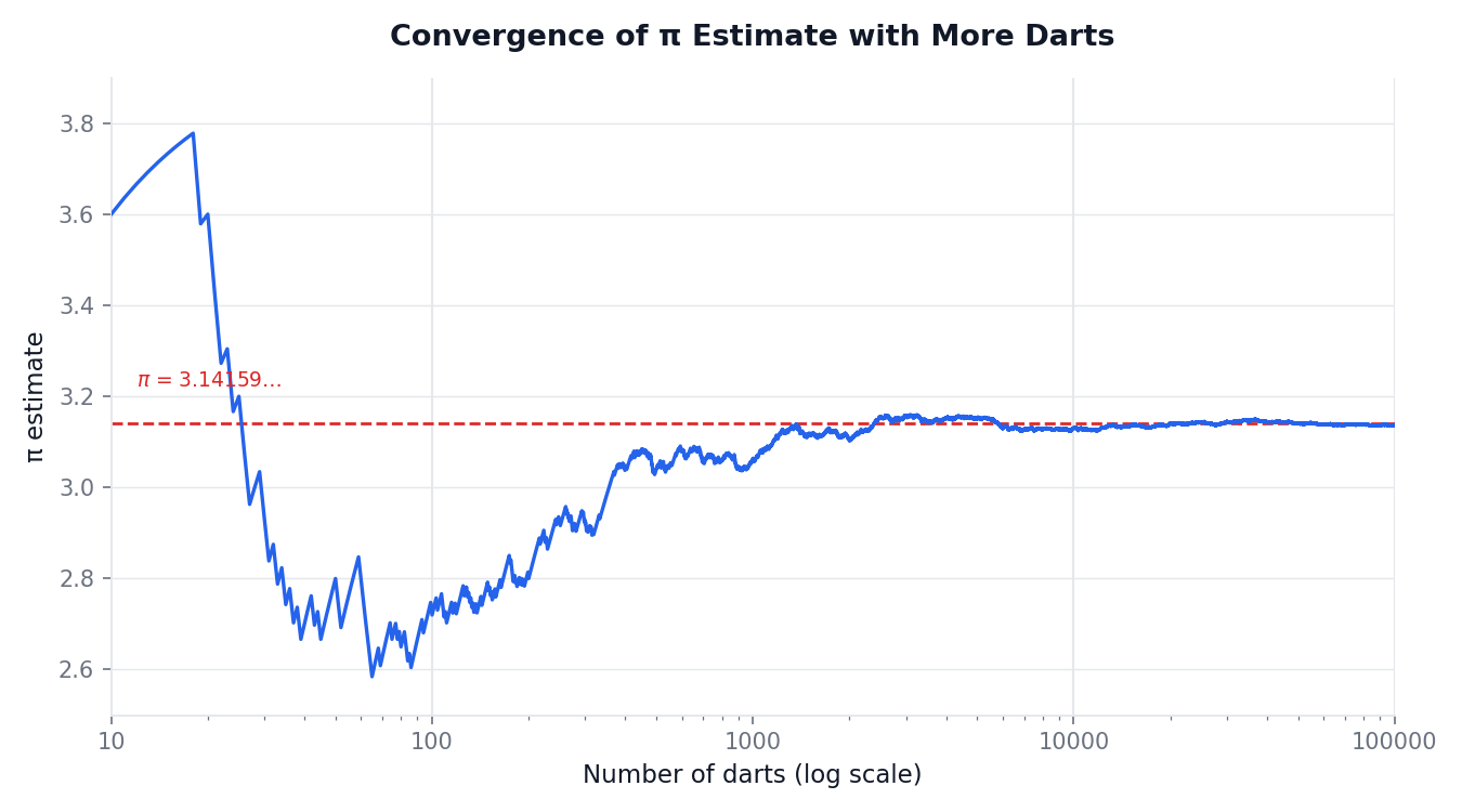
This is where a principle you have seen informally throughout the learning path becomes especially clear. When we repeat a random experiment many times, the observed proportion of a particular outcome tends to settle closer and closer to the true probability. This idea is often called the law of large numbers.

Consider two simulation runs side by side:

Simulation	Total darts	Darts inside	Proportion inside	π estimate
Run A	100	73	0.7300	2.920
Run B	100,000	78,502	0.78502	3.14008

Run A's estimate is noticeably off, while Run B lands remarkably close to the true value of $\pi \approx 3.14159$ . With only 100 darts, random variation can easily push the count a few points in either direction. With 100,000 darts, those random wobbles mostly cancel each other out, and the proportion locks in near $\frac{\pi}{4}$ .

Line plot showing the π estimate converging toward true π as the number of darts increases

Think of it like a poll: asking 10 people for their opinion can give a misleading picture, but surveying 10,000 people produces a result you can trust. The same logic applies here — more darts mean more information, which means the randomness averages out and our estimate sharpens.

Let's recap the full simulation in a few clear steps:

Draw the setup. Place a quarter-circle of radius 1 inside a unit square.
Throw random darts. Each dart lands at a random point $(x, y)$ where $0 \leq x \leq 1$ and $0 \leq y \leq 1$ .
Check each dart. A dart is inside the quarter-circle if $x^2 + y^2 \leq 1$ .
Count and compute. Divide the number of darts inside by the total number of darts, then multiply by 4 to estimate $\pi$ .

The beauty of this method is its simplicity. We do not need advanced geometry or calculus to get a reasonable estimate of $\pi$ — all we need is randomness, counting, and the area relationship we established earlier. It is a vivid example of how probability can reach beyond predicting outcomes and actually help us discover mathematical truths.

Estimating $\pi$ with darts is a wonderful demonstration, but you might wonder whether anyone actually uses this "throw random points and count" strategy for serious work. The answer is a resounding yes. Monte Carlo methods are one of the most widely used computational techniques in science and engineering. The core idea is always the same one we applied here: simulate a random process many times, observe what fraction of trials satisfy a condition, and use that fraction to estimate something you cannot easily calculate directly.

Here are a few real-world areas where this idea appears:

Nuclear and particle physics. Monte Carlo methods were originally developed during the Manhattan Project to model how neutrons scatter through materials — a problem with so many possible paths that exact calculation was impractical. Modern particle physicists at facilities like CERN still rely on massive Monte Carlo simulations to predict what detector signals should look like.
Climate science. Climate models contain many uncertain parameters — cloud behavior, ocean currents, ice-sheet dynamics. Researchers run thousands of simulations with randomly sampled parameter values to estimate the range of plausible future temperatures, essentially asking "what fraction of scenarios lead to more than 2°C of warming?"
Medicine and drug design. When modeling how a drug molecule interacts with a protein, scientists randomly sample molecular shapes and orientations to estimate binding strength. The fraction of configurations that "fit" gives an estimate of how effective the drug might be.
Finance. Banks and investment firms simulate thousands of random market scenarios to estimate the probability that a portfolio will lose more than a certain amount, a measure known as Value at Risk.

In every case, the pattern matches what we did: define a space, generate random samples, check a condition, and turn the observed proportion into a useful estimate. The $\pi$ dartboard is simply the most intuitive entry point into a technique that powers some of the most complex computations on the planet.

In this lesson, we saw that a quarter-circle inscribed in a unit square has an area of $\frac{\pi}{4}$ , which means a randomly thrown dart has a probability of $\frac{\pi}{4}$ of landing inside the curve. By flipping that relationship around, we can estimate $\pi$ as $4 \times \frac{\text{darts inside}}{\text{total darts}}$ , and the estimate improves as we increase the number of throws — a hands-on glimpse of the law of large numbers in action. We also saw that this same Monte Carlo logic extends far beyond our dartboard, powering real discoveries in physics, climate science, medicine, and finance.

This wraps up the final lesson of the course and, in fact, the entire learning path. In the upcoming practice tasks, you will compute π estimates from simulated dart data, compare the absolute errors of different runs, and identify why larger sample sizes consistently produce more accurate results. Let's finish strong!