Greetings, and welcome to the exciting lesson on Comparing Different Optimizers for Autoencoders! In prior lessons, we've learned about Autoencoders, their role in dimensionality reduction, elements like loss functions, and optimizers. Now, it's time to apply this knowledge and delve deeper into the fascinating world of optimizers.

In this lesson, we will train our Autoencoder using different optimizers and then compare their performance based on the reconstruction error. Our goal? To understand how different optimizers can impact the Autoencoder's ability to reconstruct its inputs.

Recalling from our previous lessons, optimizers in machine learning algorithms are used to update and adjust model parameters, reducing errors. These errors are defined by loss functions, which estimate how well the model is performing its task. Some commonly used optimizers include Stochastic Gradient Descent (SGD), Adam, RMSprop, and Adagrad. Although they all aim to minimize the loss function, they do so in different ways, leading to variations in performance. Understanding these differences enables us to choose the best optimizer for our machine learning tasks.

As a starting point, we need an Autoencoder, but before moving there, let's generate a dataset using the mlbench package. We'll use the mlbench.waveform dataset, which is suitable for demonstrating dimensionality reduction:

Next, we define a simple Autoencoder with a Dense input layer and a Dense output layer; both layers have the same dimensions:

This R function creates a simple Autoencoder using keras3. The function accepts the dimensions of the input layer, the encoded layer, and the optimizer as arguments. In the end, it compiles the Autoencoder with the specified optimizer and binary_crossentropy as the loss function.

After the model structure is defined, we train the Autoencoder on the dataset and evaluate its performance using the reconstruction error. Here, the reconstruction error is the mean squared error between the original data (input) and the reconstructed data (output):

Next, we compare the performance of different optimizers by training our Autoencoder with each optimizer and computing the corresponding reconstruction error:

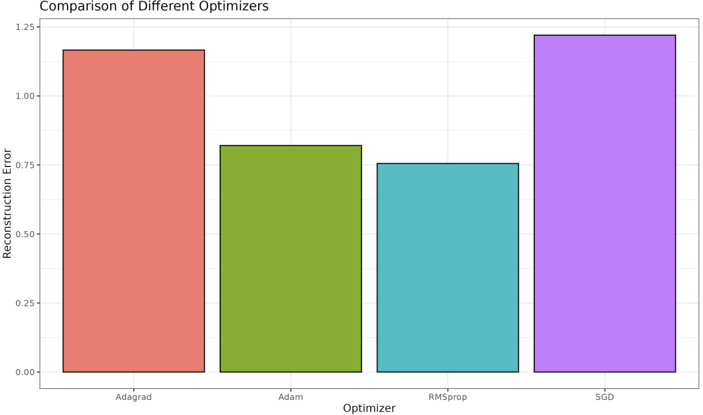
In the above code, we first initialize a list with the optimizers we want to compare: SGD, Adam, RMSprop, and Adagrad. Next, we train our Autoencoder using each optimizer, compute the reconstruction error, and store the results for comparison.

Lastly, we visualize the results using a bar plot to effectively compare the optimizers. We assign the plot to a variable and use a white background for clarity:

Through this plot, we can observe the impact of different optimizers on the Autoencoder's training.

In sum, we've trained an Autoencoder using different optimizers (Stochastic Gradient Descent, Adam, RMSprop, and Adagrad), assessed their impact on the model, and compared them visually. By the end of the upcoming exercise, you'll have not only a firm understanding of how different optimizers work but also a hands-on understanding of their effects on an Autoencoder's performance. Have fun experimenting!