Welcome back to Drawing Conclusions from a Sample! With five of seven lessons now underway, you are in the home stretch. Over the previous lessons you learned to estimate population means and proportions from random samples, and last time you discovered that pulling a different random sample almost always gives a different estimate — a phenomenon called sampling variability. That insight raised an unavoidable practical question: if we can only collect one sample, how confident should we be in the number it produces? This lesson gives you a concrete way to answer that question by measuring the spread of many possible estimates and using it to express the likely error of a single one.
From Noticing Variation to Measuring It
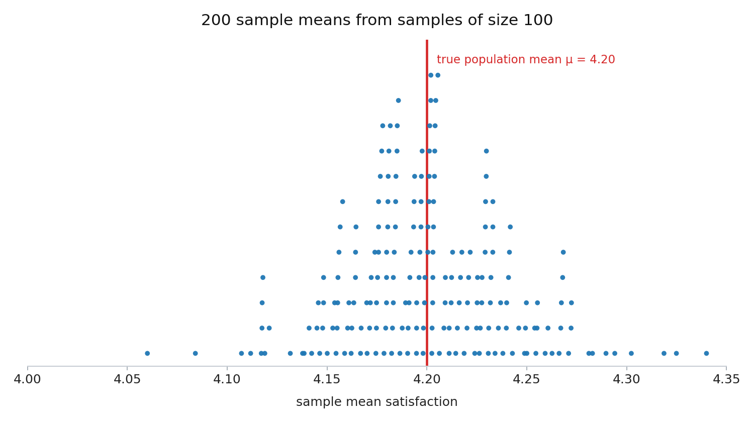
In the last lesson, we pictured sampling variability as a cloud of dots — each dot a sample estimate — clustered around the true population value. That image told us something reassuring: estimates do not fly off in random directions; they stay relatively close to the truth.
Today, we take the next step: measuring the width of that cloud. A tight cloud means any single estimate is probably very close to the true value. A wide cloud means an estimate could be farther off. Quantifying that width turns a vague feeling of "close enough" into a number we can report alongside our estimate, giving anyone who reads it a realistic sense of how much trust to place in it.
Building the Cloud with Simulated Samples
To see the cloud take shape, let's return to the online retailer with 50,000 customers and a true mean satisfaction rating of μ=4.20. This time, imagine we draw not three samples but 200 independent random samples, each of size 100, and compute the sample mean xˉ for every one.
Here are the first five of those 200 means:
Sample
xˉ
1
4.17
2
4.23
3
4.14
4
4.25
5
4.21
Across all 200 means, the values range from roughly 4.06 to 4.34, but the vast majority land between about 4.10 and 4.30. That spread is not just noise — it is real, measurable information we can put to work.
Join the 1M+ learners on CodeSignal
Be a part of our community of 1M+ users who develop and demonstrate their skills on CodeSignal
Measuring the Typical Distance from the Truth
Turning the Spread into a Plausible Range
Stating an Estimate with Uncertainty
Larger Samples Shrink the Spread
Conclusion and Next Steps
In this lesson, you moved from simply knowing that estimates vary to measuring that variation and putting it to work. By computing how far sample estimates typically land from the true value, you gained a concrete way to express uncertainty — a plausible range built from the point estimate and the typical estimation error. You also saw that increasing the sample size tightens that range, giving you more precision when you need it.
Now it is time to practice. In the exercises ahead, you will generate your own clouds of estimates, watch the spread respond to different sample sizes, and write uncertainty statements that pair an estimate with a realistic sense of how far off it might be. Let's get started!
A natural way to summarize how spread out the cloud is relies on a tool you already know from the Summarizing Sample Data course: the mean absolute deviation (MAD). Previously, you used MAD to describe how far individual data points typically sit from a sample mean. Here, we apply the exact same idea on a different level — we measure how far the sample means themselves typically sit from the true population meanμ.
The process is straightforward. Take each of the 200 sample means, find its absolute distance from μ=4.20, and then average those distances. Suppose the result is about 0.05. That single number tells us that a typical sample mean lands roughly 0.05 away from the truth. We will call this the typical estimation error.
This answers a very practical question: when we draw one random sample of 100 customers and compute xˉ, we should expect to miss the true mean by about 0.05 in either direction.
Here is where the payoff arrives. Suppose we have drawn just one sample of 100 customers and obtained xˉ=4.18. We do not know μ, but we know from simulations (or past experience with similar surveys) that the typical estimation error for samples of this size is about 0.05.
The typical error is a rough uncertainty measure, not a formal guarantee. A simple way to communicate it is to place that amount on either side of our estimate. That gives us a rough plausible range:
plausible range=xˉ±typical error=4.18±0.05
So we would report a rough plausible range from 4.13 to 4.23. This is not a guarantee or a formal confidence interval — the true value could fall outside this window — but it gives a concise way to describe typical sampling uncertainty around the estimate. The same arithmetic applies when estimating a population proportion: add and subtract the typical error around p^ to form a rough plausible range.
Whenever we report a sample estimate, pairing it with a statement of uncertainty makes it far more informative. Compare these two reports:
Report Style
Statement
Without uncertainty
"The average customer satisfaction is about 4.18."
With uncertainty
"We estimate that the average customer satisfaction is about 4.18, give or take roughly 0.05."
The second version is both more honest and more useful. It tells the reader that the true value could reasonably be a little higher or a little lower, and it quantifies how much higher or lower. A useful rough uncertainty statement always combines two ingredients: the point estimate (the single number from the sample, such as xˉ=4.18) and a measure of likely error, expressed as "give or take 0.05," "within about 0.05," or as an explicit range like "between 4.13 and 4.23."
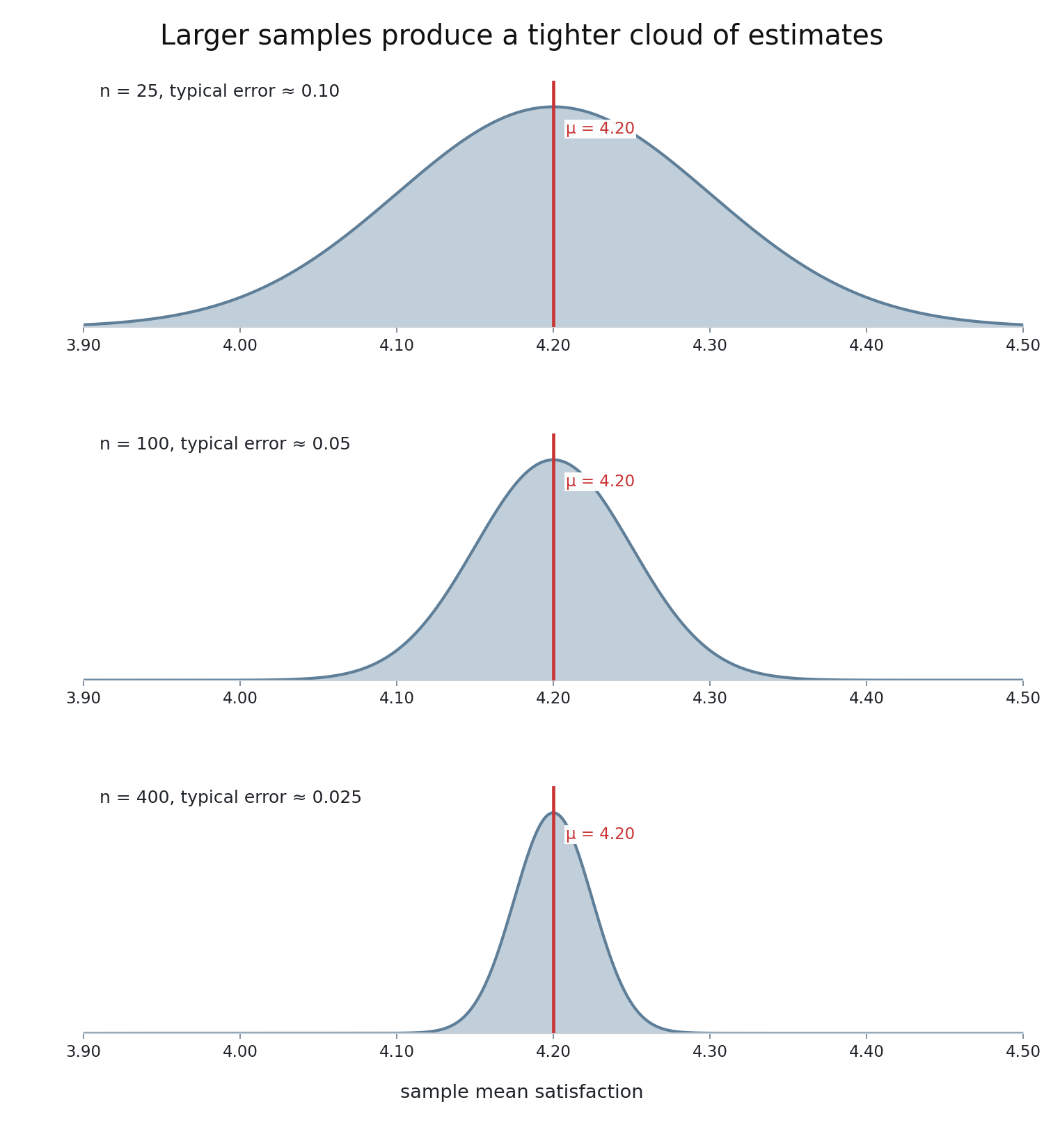
One more idea deserves attention. The typical estimation error is not a fixed number — it depends on sample size. When each sample includes more people, it captures more of the population's diversity, so the sample means bunch together more tightly around μ.
Consider how the typical error changes for our retailer scenario as we increase n:
Sample Size (n)
Typical Error (approx.)
Plausible Range around xˉ
25
0.10
xˉ±0.10
100
0.05
xˉ±0.05
400
0.025
xˉ±0.025
The visual below shows this effect clearly — the cloud of sample means tightens as sample size grows:
The takeaway is direct: bigger samples produce a tighter cloud of estimates and therefore a smaller likely error. If an estimate's uncertainty feels too large for the decision at hand, collecting a larger sample is the most straightforward way to reduce it.