Cohort Trend Comparisons

Welcome back to Comparing Rows with LEAD and LAG. We are now in Lesson 4 of 4. In the previous lesson, we compared one overall monthly series with its preceding month. Now we will keep that aggregate, then compare its pattern across several monthly series at once.

Instead of grouping all customers together, we will group customers by the month in which they signed up. Then we will:

• Assign each customer to a signup month cohort.
• Calculate gross order value for each cohort and sales month.
• Compare adjacent populated months inside each cohort with window functions.

By the end, we will have a complete cohort trend report built from three focused CTE stages.

A regular monthly comparison asks, “How did this month compare with the previous month?” A cohort analysis asks that question separately for each customer group. For example, customers who signed up in January 2021 form one cohort, while customers who signed up in February 2021 form another.

Each cohort becomes its own ordered timeline. The same sales month can appear on several rows because different cohorts may have orders during that month. This means we must control the row grain carefully:

1. One row per customer in the cohort assignment stage.
2. One row per cohort and populated sales month in the aggregation stage.
3. One row per cohort and sales month with neighboring values in the trend stage.

As in earlier lessons, we compare rows only after creating the correct summarized grain.

We begin with the Customers table and convert each signup_date into the first day of its month. DATE_FORMAT creates the YYYY-MM-01 form, while CAST(... AS DATE) gives us a true date value that is easy to group and sort. The following query makes the first CTE visible on its own.

WITH customer_cohorts AS (
    SELECT
        customer_id,
        CAST(DATE_FORMAT(signup_date, '%Y-%m-01') AS DATE) AS cohort_month
    FROM Customers
)
SELECT
    customer_id,
    cohort_month
FROM customer_cohorts
ORDER BY cohort_month, customer_id;

The customer_cohorts CTE gives every customer exactly one cohort_month. Because each customer has one customer_id, the final ordering by cohort month and customer ID is deterministic. The dataset also guarantees that every signup date comes before that customer’s first order, so assigning later orders to this cohort is safe. A customer’s cohort reflects when the customer joined, not when the customer first purchased.

Next, we connect each customer cohort to its orders, order items, and products. The order date supplies the sales month, while each order item contributes quantity * product_price to the monthly total. The query below includes the cohort stage and adds the monthly aggregation stage so it can run independently.

WITH customer_cohorts AS (
    SELECT
        customer_id,
        CAST(DATE_FORMAT(signup_date, '%Y-%m-01') AS DATE) AS cohort_month
    FROM Customers
),
cohort_monthly_order_value AS (
    SELECT
        cc.cohort_month,
        CAST(DATE_FORMAT(o.order_date, '%Y-%m-01') AS DATE) AS sales_month,
        SUM(oi.quantity * p.product_price) AS monthly_order_value
    FROM customer_cohorts AS cc
    INNER JOIN Orders AS o
        ON o.customer_id = cc.customer_id
    INNER JOIN OrderItems AS oi
        ON oi.order_id = o.order_id
    INNER JOIN Products AS p
        ON p.product_id = oi.product_id
    GROUP BY
        cc.cohort_month,
        sales_month
)
SELECT
    cohort_month,
    sales_month,
    monthly_order_value
FROM cohort_monthly_order_value
ORDER BY cohort_month, sales_month;

The joins follow the data path from customers to orders, then to order items and products. The GROUP BY creates one row for each cohort month and populated sales month pair. The CTE and column use the provided name monthly_order_value, but we interpret this metric as gross order value.

The database has no stored order total or transaction-time price, so current catalog prices are a deliberate proxy. No order_status filter is applied, which means canceled and refunded orders remain included. Therefore, this value should not be treated as recognized order value or customer spend.

The aggregation stage now gives us comparison-ready rows. Although MySQL can accept LAG() or LEAD() without a window ORDER BY, previous and next rows are not meaningfully or deterministically defined without one, so always provide an ORDER BY for chronological comparisons. We partition by cohort_month so comparisons restart for every signup cohort, then order each partition by sales_month.

WITH customer_cohorts AS (
    SELECT
        customer_id,
        CAST(DATE_FORMAT(signup_date, '%Y-%m-01') AS DATE) AS cohort_month
    FROM Customers
),
cohort_monthly_order_value AS (
    SELECT
        cc.cohort_month,
        CAST(DATE_FORMAT(o.order_date, '%Y-%m-01') AS DATE) AS sales_month,
        SUM(oi.quantity * p.product_price) AS monthly_order_value
    FROM customer_cohorts AS cc
    INNER JOIN Orders AS o
        ON o.customer_id = cc.customer_id
    INNER JOIN OrderItems AS oi
        ON oi.order_id = o.order_id
    INNER JOIN Products AS p
        ON p.product_id = oi.product_id
    GROUP BY
        cc.cohort_month,
        sales_month
),
cohort_trends AS (
    SELECT
        cohort_month,
        sales_month,
        monthly_order_value,
        LAG(monthly_order_value) OVER (
            PARTITION BY cohort_month
            ORDER BY sales_month
        ) AS previous_month_order_value,
        LEAD(monthly_order_value) OVER (
            PARTITION BY cohort_month
            ORDER BY sales_month
        ) AS next_month_order_value
    FROM cohort_monthly_order_value
)
SELECT
    cohort_month,
    sales_month,
    previous_month_order_value,
    monthly_order_value,
    next_month_order_value
FROM cohort_trends
ORDER BY cohort_month, sales_month;

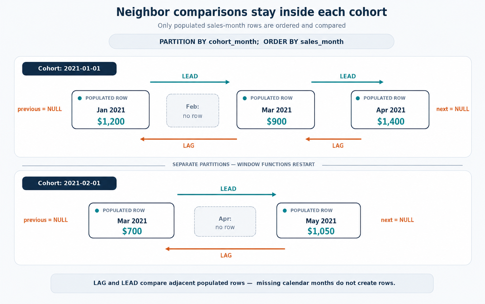
LAG() retrieves the value from the previous populated row in the same cohort. LEAD() retrieves the value from the next populated row in that cohort. At the first row of a cohort, LAG() returns NULL; at the last row, LEAD() returns NULL. We preserve these values because no comparison exists at those edges.

These functions compare populated rows, not automatically generated calendar months. If a cohort has sales in January and March but no sales in February, January and March are still adjacent rows in that cohort. This report does not fill missing calendar periods.

The following diagram shows how neighboring-row comparisons stay inside each cohort and can cross an unpopulated calendar month.

The final step is to present the cohort and sales months together with the three monetary values. We apply ROUND(..., 2) in the outer query after the window comparisons have been calculated. This formats the displayed values without changing the values used by LAG() and LEAD(). Rounding a missing value still returns NULL, so unavailable comparisons remain visible.

Here is the complete, runnable MySQL 8.0 query:

WITH customer_cohorts AS (
    SELECT
        customer_id,
        CAST(DATE_FORMAT(signup_date, '%Y-%m-01') AS DATE) AS cohort_month
    FROM Customers
),
cohort_monthly_order_value AS (
    SELECT
        cc.cohort_month,
        CAST(DATE_FORMAT(o.order_date, '%Y-%m-01') AS DATE) AS sales_month,
        SUM(oi.quantity * p.product_price) AS monthly_order_value
    FROM customer_cohorts AS cc
    INNER JOIN Orders AS o
        ON o.customer_id = cc.customer_id
    INNER JOIN OrderItems AS oi
        ON oi.order_id = o.order_id
    INNER JOIN Products AS p
        ON p.product_id = oi.product_id
    GROUP BY
        cc.cohort_month,
        sales_month
),
cohort_trends AS (
    SELECT
        cohort_month,
        sales_month,
        monthly_order_value,
        LAG(monthly_order_value) OVER (
            PARTITION BY cohort_month
            ORDER BY sales_month
        ) AS previous_month_order_value,
        LEAD(monthly_order_value) OVER (
            PARTITION BY cohort_month
            ORDER BY sales_month
        ) AS next_month_order_value
    FROM cohort_monthly_order_value
)
SELECT
    cohort_month,
    sales_month,
    ROUND(previous_month_order_value, 2) AS previous_month_order_value,
    ROUND(monthly_order_value, 2) AS monthly_order_value,
    ROUND(next_month_order_value, 2) AS next_month_order_value
FROM cohort_trends
ORDER BY cohort_month, sales_month;

The three CTEs each have one clear responsibility: customer_cohorts assigns signup groups, cohort_monthly_order_value calculates one monthly value per cohort, and cohort_trends adds neighboring values. The outer query formats the result. Because the aggregated grain contains at most one row for each cohort and sales month pair, ORDER BY cohort_month, sales_month provides a deterministic final order.

In this lesson, we changed the reporting perspective from one overall monthly timeline to several customer timelines organized by signup month. We used DATE_FORMAT and CAST to assign each customer to a cohort, joined through orders and order items to calculate gross order value, and grouped the data by cohort month and sales month.

After aggregation, we used LAG() and LEAD() with PARTITION BY cohort_month and ORDER BY sales_month. The functions restart for every cohort, compare adjacent populated rows, and preserve NULL when a previous or next row does not exist. This is the final lesson in the course, and reaching the end of this lesson sequence shows the progress we have made with CTEs and window functions.

In the practice section, we will observe a related category trend, build a country activity trend, and then complete the cohort report independently, turning this pattern into confident SQL work.