Cluster Validation in R

Welcome! In today's lesson, we'll delve into cluster validation. We will interpret and implement the Silhouette Score and learn how to visualize clusters for validation in R. All of these concepts form a unified understanding that we'll explore.

Cluster validation, a key step in Cluster Analysis, involves evaluating the quality of the outcomes of the clustering process. Proper validation helps avoid common issues such as overfitting or misjudging the optimal number of clusters.

One metric that plays a crucial role in cluster validation is the Silhouette Score. This measure quantifies the quality of clustering, providing an indication of how well each data point resides within its cluster. The Silhouette Score $s(i)$ for a sample $i$ is formulated as:

$s(i) = \frac{b(i) - a(i)}{max\{a(i), b(i)\}}$

Here, $a(i)$ represents the average intra-cluster distance, and $b(i)$ signifies the mean nearest-cluster distance.

Knowing how to interpret the Silhouette Score is essential. The Silhouette Score ranges between -1 and 1. The value of the Silhouette Score has the following interpretation:

• Score close to 1: The item is well-matched to its own cluster and poorly matched to neighboring clusters. This would be an indication of strong clustering.

• Score close to 0: The item is on or very close to the decision boundary between two neighboring clusters. The data point is right at the boundary of the clusters. It's not distinctly in one cluster or another. Here, our clustering model is uncertain about the assignment of these points.

• Score close to -1: The item is mismatched to its own cluster and matched to a neighboring cluster. This case indicates that we've likely assigned a point to the wrong cluster, as it is closer to the neighboring cluster than its own.

Ideally, all objects would have a Silhouette Score of 1, but in practice, it’s almost impossible.

Let's implement the Silhouette Score in R step by step. We'll start by defining helper functions for distance calculations and then compute the Silhouette Score.

First, we define a function to calculate the Euclidean distance between two points:

euclidean_distance <- function(a, b) {
  sqrt(sum((a - b)^2))
}

Next, we define a function to calculate $a(i)$, the average distance from a point to all other points in the same cluster:

calculate_a <- function(point, cluster) {
  if (nrow(cluster) <= 1) {
    return(0)
  }
  distances <- apply(cluster, 1, function(other) euclidean_distance(point, other))
  # Remove the distance to itself (should be zero)
  distances <- distances[distances != 0]
  mean(distances)
}

Now, we define a function to calculate $b(i)$, the lowest average distance from a point to all points in other clusters:

calculate_b <- function(point, clusters, current_cluster_idx) {
  min_avg_dist <- Inf
  for (i in seq_along(clusters)) {
    if (i == current_cluster_idx) next
    cluster <- clusters[[i]]
    distances <- apply(cluster, 1, function(other) euclidean_distance(point, other))
    avg_dist <- mean(distances)
    if (avg_dist < min_avg_dist) {
      min_avg_dist <- avg_dist
    }
  }
  min_avg_dist
}

Finally, we define a function to compute the silhouette score for each data point and the average silhouette score:

custom_silhouette_score <- function(data, labels) {
  clusters <- split(as.data.frame(data), labels)
  clusters <- lapply(clusters, as.matrix)
  scores <- numeric(nrow(data))
  for (i in 1:nrow(data)) {
    point <- as.numeric(data[i, ])
    label <- labels[i]
    cluster_idx <- which(names(clusters) == label)
    a <- calculate_a(point, clusters[[cluster_idx]])
    b <- calculate_b(point, clusters, cluster_idx)
    if (max(a, b) > 0) {
      scores[i] <- (b - a) / max(a, b)
    } else {
      scores[i] <- 0
    }
  }
  mean(scores)
}

For visualization, we will use ggplot2 to plot the clusters. Now, let's observe the implementation of our functions using the Iris dataset. We'll calculate the Silhouette Score for the k-means clustering model. First, let's perform the clustering and visualize the clusters:

library(ggplot2)
data(iris)

# Use only the numeric columns for clustering
X <- iris[, 1:4]

# Fit the k-means model
set.seed(0)
kmeans_model <- kmeans(X, centers = 3, nstart = 10)

# Add cluster labels to the data
iris$Cluster <- as.factor(kmeans_model$cluster)

# Compute the first two principal components
pca <- prcomp(X)
pc_data <- as.data.frame(pca$x[, 1:2])
pc_data$Cluster <- iris$Cluster

# Visualize the clusters using ggplot2
ggplot(pc_data, aes(x = PC1, y = PC2, color = Cluster)) +
  geom_point(size = 2, alpha = 0.7) +
  labs(title = "K-means Clustering on Iris Data (First 2 Principal Components)",
       x = "PC1", y = "PC2") +
  theme_minimal()

Output:

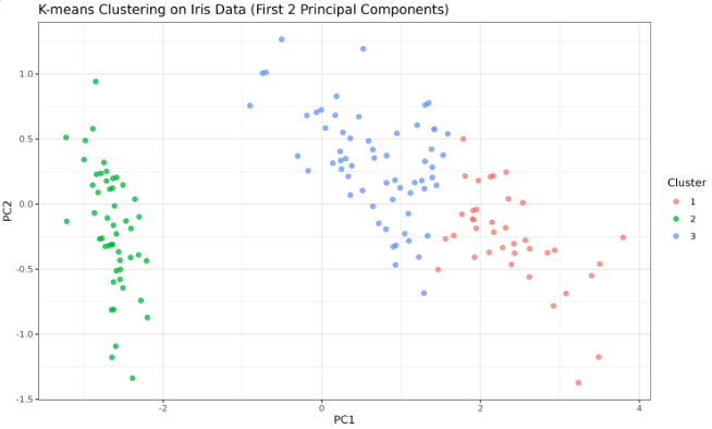
The plot will show the clusters formed by the k-means model. Note that the plot may look different depending on the random seed and R version.

Now, let's calculate the Silhouette Score using our custom implementation:

# Calculate and print the average silhouette score
average_score <- custom_silhouette_score(X, kmeans_model$cluster)
cat(sprintf("Silhouette Score (Custom): %.2f\n", average_score)) # ~0.55

R provides built-in functions to compute the Silhouette Score, such as the silhouette function from the cluster package. This function requires the cluster assignments and a distance matrix.

Here's how to use it:

library(cluster)

# Compute the distance matrix
diss <- dist(X)

# Compute the silhouette object
sil <- silhouette(kmeans_model$cluster, diss)

# Average silhouette width
avg_sil_width <- mean(sil[, 3])
cat(sprintf("Silhouette Score (cluster package): %.2f\n", avg_sil_width)) # ~0.55

Great job! We've successfully covered the theory of cluster validation, the mathematics and practical application of the Silhouette Score, and visualized clusters using R. Now, prepare for some practical exercises to solidify your understanding and boost your confidence. Happy learning!