Welcome to Building Probability Models, the third course in your learning path! In the first two courses, you explored what probability means, learned how to identify sample spaces and outcomes, and discovered how experimental data can estimate the likelihood of events. That foundation puts you in a great position for what comes next: learning how to build, use, and evaluate probability models.

In this first lesson, we will look at what a probability model actually is and, more importantly, what makes one valid. By the end, you will be able to check any set of outcome–probability pairs and confidently say whether it qualifies as a proper probability model.

As you may recall from previous courses, every chance process has a sample space, which is the complete list of possible outcomes. For example, when you roll a standard six-sided die, the sample space is $\{1, 2, 3, 4, 5, 6\}$. You also learned that each outcome can be assigned a probability, and that experimental data (relative frequency) can help us estimate those probabilities.

A probability model takes this one step further. Instead of just listing outcomes, it pairs every outcome in the sample space with a specific probability value. Think of it as a complete blueprint that tells us how likely each possible result is before any experiment is run.

So what rules must that blueprint follow to be considered valid? That is exactly what we will unpack next.

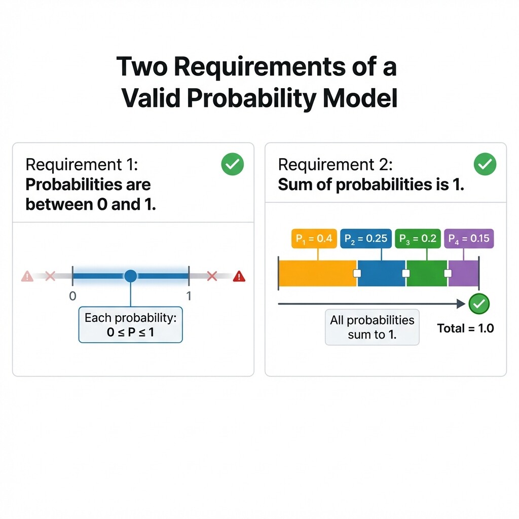
A valid probability model must satisfy exactly two requirements:

1. Every probability is between 0 and 1 (inclusive). Each outcome's assigned probability $P$ must satisfy $0 \le P \le 1$. A probability of $0$ means the outcome is impossible, and a probability of $1$ means it is certain. Negative numbers or values greater than do not make sense as probabilities.

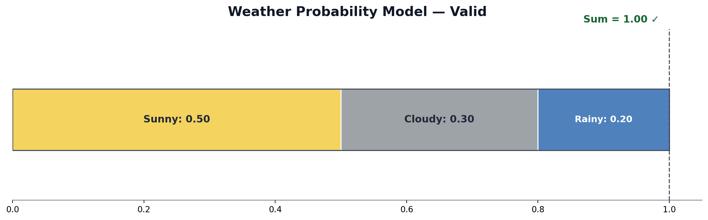
Let us see the two requirements in action. Suppose a weather app models tomorrow's conditions using three outcomes: Sunny, Cloudy, and Rainy. The app assigns the following probabilities:

Requirement 1: Every probability is between $0$ and $1$. The values , , and all pass this check.

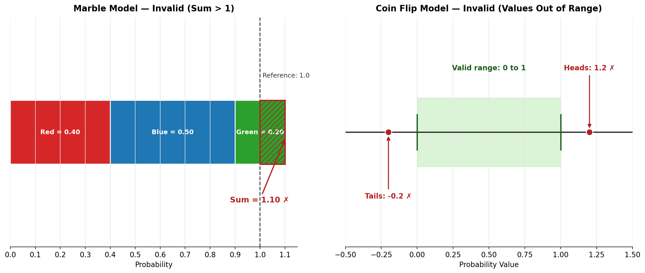
Now let us look at models that fail one or both requirements. Consider a model for drawing a marble from a bag containing red, blue, and green marbles:

Each individual probability is between $0$ and $1$, so Requirement 1 is satisfied. But the sum tells a different story:

You might wonder why we insist on these two rules so strictly. The reason is practical: a probability model is meant to predict real outcomes. If a probability were negative, it would suggest something less likely than impossible, which has no real-world meaning. If probabilities summed to more or less than $1$, our model would claim that total chance is either too much or too little, leaving gaps or overlaps in our predictions.

When a model satisfies both requirements, we can trust it as a reliable starting point for making predictions. Later in this course, you will use valid models to forecast how often each outcome should appear over many trials and then compare those forecasts with observed data. Getting the foundation right here makes everything that follows more meaningful.

Let us recap the key ideas. A valid probability model pairs every outcome in the sample space with a probability and must pass two checks: each probability is between $0$ and $1$, and all probabilities add up to exactly $1$. If either rule is broken, the model is invalid, no matter how reasonable it might look at first glance.

Up next, you will put these ideas into action with a set of hands-on practice tasks. You will judge whether models are valid, diagnose exactly which rule an invalid model violates, and even fill in missing probabilities to repair a broken model. These exercises will sharpen your ability to verify probability models quickly and confidently.