Modular Training Components

Introduction

Welcome to lesson 2 of "Building and Applying Your Neural Network Library"! In the previous lesson, you took your first steps toward a professional-grade neural network library by modularizing your core components — dense layers and activation functions — using a modern JavaScript project structure and ES modules. You learned how to organize your codebase for maintainability and extensibility, setting the stage for a robust machine learning framework. Now, it's time to take the next big step: modularizing your training components . In neural network training, two essential elements beyond the layers themselves are loss functions (which measure how well the network is performing) and optimizers (which update the network's weights based on computed gradients). If these components are scattered throughout your code, it becomes difficult to reuse, test, or extend them. In this lesson, you'll organize these training components into dedicated modules within your neuralnets project. You'll create a losses submodule to house your Mean Squared Error (MSE) loss function and an optimizers submodule for your Stochastic Gradient Descent (SGD) optimizer. By the end, you'll have a fully modular training pipeline that demonstrates the power of good software architecture in JavaScript-based machine learning projects.

Our Test Dataset: The XOR Problem

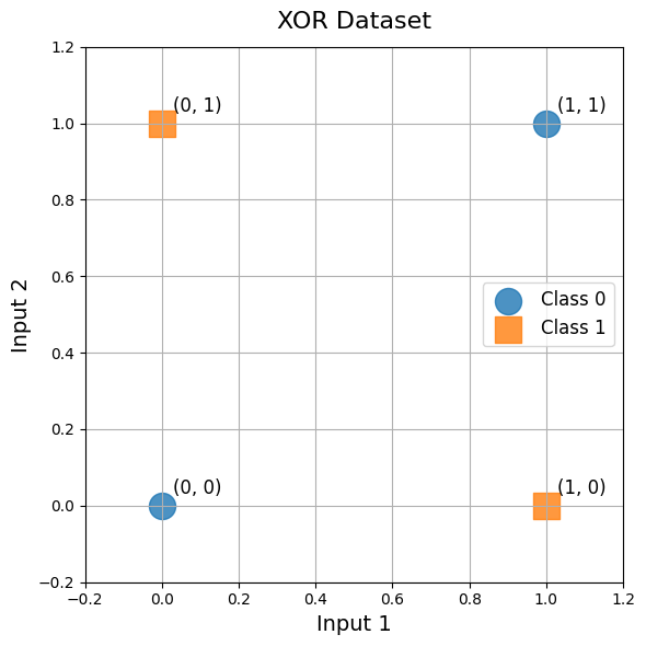
Before we dive into modularizing our training components, let's look at the dataset we'll use to test our library: the XOR (exclusive OR) problem . This is a classic example in machine learning, perfect for testing neural networks because it cannot be solved by a simple linear model — it requires a network with at least one hidden layer. The XOR problem consists of four data points, each with two binary inputs and one binary output. The output is 1 when exactly one of the inputs is 1 and 0 otherwise. The pattern looks like this: [0,0] \to 0, [0,1] \to 1, [1,0] \to 1, [1,1] \to 0 . While XOR is often treated as a classification problem, we'll frame it as a regression task by using the mean squared error loss. Here's how you can set up the XOR dataset in JavaScript using mathjs : JavaScript import * as math from 'mathjs'; // XOR dataset setup const X_train = math.matrix([[0, 0], [0, 1], [1, 0], [1, 1]]); const y_train = math.matrix([[0], [1], [1], [0]]); We'll use this simple dataset for rapid development and testing. Later in the course, you'll apply your complete neural network library to a real-world dataset, such as the California Housing dataset, to predict house prices based on features like location, population, and median income.

Join the 1M+ learners on CodeSignal

Be a part of our community of 1M+ users who develop and demonstrate their skills on CodeSignal

Creating the Optimizers Module

Just like with loss functions, it's best practice to encapsulate your optimization algorithms in their own module. Here, you'll implement a simple Stochastic Gradient Descent (SGD) optimizer as a class, which will handle updating the weights and biases of your layers.

Create a new file for your optimizer:

neuralnets/optimizers/sgd.js

JavaScript

import * as math from 'mathjs';

export class SGD {
    constructor(learningRate = 0.01) {
        this.learningRate = learningRate;
    }

    update(layer) {
        // Update layer's weights and biases using their stored gradients
        if (
            layer.weights !== undefined && layer.biases !== undefined &&
            layer.dWeights !== null && layer.dBiases !== null
        ) {
            layer.weights = math.subtract(
                layer.weights,
                math.multiply(this.learningRate, layer.dWeights)
            );
            layer.biases = math.subtract(
                layer.biases,
                math.multiply(this.learningRate, layer.dBiases)
            );
        }
    }
}

import * as math from 'mathjs';

export class SGD {
    constructor(learningRate = 0.01) {
        this.learningRate = learningRate;
    }

    update(layer) {
        // Update layer's weights and biases using their stored gradients
        if (
            layer.weights !== undefined && layer.biases !== undefined &&
            layer.dWeights !== null && layer.dBiases !== null
        ) {
            layer.weights = math.subtract(
                layer.weights,
                math.multiply(this.learningRate, layer.dWeights)
            );
            layer.biases = math.subtract(
                layer.biases,
                math.multiply(this.learningRate, layer.dBiases)
            );
        }
    }
}

And create an index.js file in the optimizers folder to re-export your optimizer:

neuralnets/optimizers/index.js

JavaScript

export { SGD } from './sgd.js';

export { SGD } from './sgd.js';

Now, you can import your optimizer class anywhere in your project:

JavaScript

import { SGD } from './optimizers/index.js';

import { SGD } from './optimizers/index.js';

Building a Complete Training Pipeline

Now comes the exciting part — putting all our modular components together into a complete training pipeline! This demonstrates the power of our modular design: clean imports, specific component usage, and a readable training setup that clearly separates concerns.

Our training pipeline combines the MLP class from our previous lesson with our newly modularized loss functions and optimizers. Notice how each component has a specific responsibility: the network handles forward and backward propagation, the loss module computes objectives and gradients, and the optimizer updates weights.

neuralnets/main.js

import * as math from 'mathjs';
import { DenseLayer } from './layers/index.js';
import { mseLoss, mseLossDerivative } from './losses/index.js';
import { SGD } from './optimizers/index.js';
import { MLP } from './models/index.js';

// XOR dataset
const X_train = math.matrix([
    [0, 0],
    [0, 1],
    [1, 0],
    [1, 1]
]);
const y_train = math.matrix([
    [0],
    [1],
    [1],
    [0]
]);

// Build MLP using modular components
const mlp = new MLP();
mlp.addLayer(new DenseLayer(2, 4, 'relu'));
mlp.addLayer(new DenseLayer(4, 1, 'sigmoid'));

// Use modular optimizer
const optimizer = new SGD(0.5);

// Training loop
const epochs = 1000;
console.log(`Training MLP for XOR problem for ${epochs} epochs with LR=0.5`);

for (let epoch = 0; epoch < epochs; epoch++) {
    // 1. Forward pass
    const y_pred = mlp.forward(X_train);
    // 2. Calculate loss using modular loss function
    const loss = mseLoss(y_train, y_pred);
    // 3. Calculate gradient using modular derivative
    const dLossWrtPred = mseLossDerivative(y_train, y_pred);
    // 4. Backward pass through network
    mlp.backward(dLossWrtPred);
    // 5. Update weights using modular optimizer
    for (const layer of mlp.layers) {
        optimizer.update(layer);
    }

    if ((epoch + 1) % 200 === 0 || epoch === 0) {
        console.log(`Epoch ${String(epoch + 1).padStart(4, ' ')}/${epochs}, Loss: ${loss.toFixed(6)}`);
    }
}

// Test final performance
console.log("\n--- After Training ---");
const finalPreds = mlp.forward(X_train);
console.log("Input | True Output | Predicted Output | Rounded Prediction");
for (let i = 0; i < X_train.size()[0]; i++) {
    const input = X_train._data[i];
    const trueVal = y_train._data[i][0];
    const predVal = finalPreds._data[i][0];
    const roundedPred = Math.round(predVal);
    console.log(
        `[${input}] | ${String(trueVal).padStart(11, ' ')} | ${predVal.toFixed(4).padStart(16, ' ')} | ${String(roundedPred).padStart(18, ' ')}`
    );
}

When you run this script, you should see output similar to:

text

Training MLP for XOR problem for 1000 epochs with LR=0.5
Epoch    1/1000, Loss: 0.250048
Epoch  200/1000, Loss: 0.036447
Epoch  400/1000, Loss: 0.006105
Epoch  600/1000, Loss: 0.002965
Epoch  800/1000, Loss: 0.001892
Epoch 1000/1000, Loss: 0.001377

--- After Training ---
Input | True Output | Predicted Output | Rounded Prediction
[0,0] |           0 |           0.0580 |                  0
[0,1] |           1 |           0.9745 |                  1
[1,0] |           1 |           0.9748 |                  1
[1,1] |           0 |           0.0291 |                  0

This demonstrates that your modular neural network library can successfully learn the XOR logic, with predictions that closely match the expected outputs.

Introduction

Our Test Dataset: The XOR Problem

Join the 1M+ learners on CodeSignal

Creating the Loss Functions Module

Creating the Optimizers Module

Building a Complete Training Pipeline

Conclusion and Next Steps