Welcome back to lesson 2 of "Building and Applying Your Neural Network Library"! You've made excellent progress in this course. In our previous lesson, we successfully transformed our neural network code into a well-structured modular system by organizing our core components — dense layers and activation functions. We created clean import paths and established the foundation for a professional-grade neural network library.

Now we're ready to take the next crucial step: modularizing our training components. As you may recall from our previous courses, training a neural network involves two key components beyond the layers themselves: loss functions (which measure how well our network is performing) and optimizers (which update the network's weights based on the gradients we compute). Currently, these components are scattered throughout our training scripts, making them difficult to reuse and maintain.

In this lesson, we'll organize these training components into dedicated modules within our neuralnets directory structure. We'll create loss functions for our Mean Squared Error (MSE) loss and an optimizer class for our Stochastic Gradient Descent (SGD) optimizer. By the end of this lesson, you'll have a complete, modular training pipeline that demonstrates the power of good software architecture in machine learning projects.

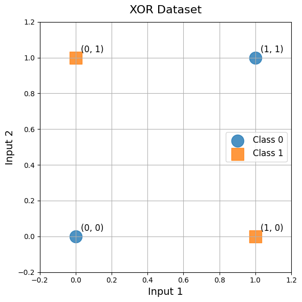
Before we dive into modularizing our training components, let's take a moment to understand the dataset we'll be using to test our library: the xor (exclusive or) problem. This is a classic toy problem in machine learning that serves as an excellent test case for neural networks because it's non-linearly separable — meaning a single linear classifier cannot solve it, but a simple multi-layer neural network can.

The xor problem consists of four data points with two binary inputs and one binary output. The output is 1 when exactly one of the inputs is 1, and 0 otherwise. This creates the pattern: [0,0] → 0, [0,1] → 1, [1,0] → 1, [1,1] → 0. This is typically treated as a classification problem, but we can frame it as a regression task as well, which is what we'll do by using our mse loss. Despite its simplicity, if our network can learn xor, then we know our forward pass, backward pass, loss calculation, and optimization code are all functioning properly.

In this setup, nrow=4 specifies we have 4 training samples, ncol=2 indicates each sample has 2 input features, and byrow=TRUE ensures the data is filled row-by-row — meaning each row represents a complete sample. This structure follows the standard convention in machine learning where rows are samples (data points) and columns are features (input dimensions).

Let's start by organizing our loss functions into dedicated functions within our neuralnets package structure. We'll create MSE loss functions that are cleanly organized and easily importable. The key insight here is separating the mathematical operations from the training logic, creating a clean interface that makes our code more testable and allows us to easily add other loss functions in the future.

neuralnets/losses/mse.R:

To make these functions available throughout our package, we create an initialization file that sources our loss functions:

neuralnets/losses/init.R:

Similarly, let's organize our optimization algorithm into its own R6 class. We'll implement our SGD optimizer as a class that encapsulates both the learning rate parameter and the update logic, following the same R6 patterns we established in our previous lesson.

The key benefit of this modular approach is that we encapsulate the optimization logic in a reusable class with a clean interface. The update method applies the sgd update rule to any layer that has trainable parameters, making our optimizer robust and flexible.

neuralnets/optimizers/sgd.R:

We also need to create an initialization file for our optimizers:

neuralnets/optimizers/init.R:

To tie all our modular components together, we create a main initialization file that loads all our modules. This creates a clean API similar to Python's __init__.py imports, making our components easily accessible throughout the package.

neuralnets/init.R:

Now comes the exciting part — putting all our modular components together into a complete training pipeline! This demonstrates the power of our modular design: clean imports, specific component usage, and a readable training setup that clearly separates concerns.

Our training pipeline combines the MLP class from our previous lesson with our newly modularized loss functions and optimizers. Notice how each component has a specific responsibility: the network handles forward and backward propagation, the loss functions compute objectives and gradients, and the optimizer updates weights. We're using a learning rate of 0.5, which is quite high compared to typical values (like 0.01 or 0.001) — this aggressive learning rate works for the simple xor problem but would likely cause instability on more complex datasets.

neuralnets/main.R:

Our neural network library now follows a clean modular architecture:

This structure provides clear separation of concerns, making our code more maintainable and allowing us to easily extend functionality. Each module has a specific purpose, and the initialization system ensures all components are properly loaded and available when needed.

When we run our complete training pipeline, we can observe how our modular neural network library learns to solve the xor problem. The training output demonstrates both the learning process and the final performance of our network:

The output shows excellent convergence — our loss decreases steadily from 0.25 to just 0.0014 over 1000 epochs. More importantly, the final predictions demonstrate that our network has successfully learned the xor logic: it outputs values close to 0 for inputs [0,0] and [1,1], and values close to 1 for inputs [0,1] and [1,0]. When rounded, these predictions perfectly match the expected xor outputs, confirming that our modular library components work together seamlessly.

The key aspects of our training pipeline that make this possible:

1. Modular Loss Functions: Our mse_loss and functions provide clean interfaces for computing objectives and gradients

Excellent work! We've successfully completed the next major step in building our neural network library by modularizing our training components. We've organized our loss functions and optimizers into dedicated modules with a clean directory structure, creating a separation of concerns that makes our code more maintainable, testable, and extensible. The successful training on the xor problem validates that our modular components work together seamlessly, setting us up perfectly for the next phase of development.

Looking ahead, we have two exciting milestones remaining in our library-building journey:

• In our next lesson, we'll create a high-level Model orchestrator class that will provide an even cleaner interface for defining, training, and evaluating neural networks.
• After that, we'll put our completed library to the test on the california housing dataset, demonstrating its capabilities on real-world regression problems.
• But first, it's time to get hands-on! The upcoming practice section will give you the opportunity to extend and experiment with the modular components we've built, reinforcing your understanding through practical application.