Welcome back to Bayesian Reasoning in the Real World! This is the second lesson out of seven in this course, and the Bayesian toolkit you have been building is about to meet one of its most consequential applications. In the previous lesson, we watched a spam filter combine several weak word-level cues into a strong verdict by chaining Bayesian updates. Today we move from the inbox to the courtroom, where a closely related reasoning error can carry far higher stakes.
In criminal trials, forensic evidence such as DNA profiles or fingerprint matches is often presented alongside very small probabilities. Those small numbers can sound airtight to a jury, but a subtle misreading of what they actually mean has led to real-world miscarriages of justice. Let's look at how probability evidence is sometimes misused in legal arguments and how Bayes' theorem sets the record straight.
When Small Probabilities Feel Like Proof
Imagine a prosecutor stands before a jury and declares: "The chance of this forensic evidence matching an innocent person is only 1 in 10,000. Therefore, there is only a 1 in 10,000 chance the defendant is innocent." That sounds compelling — a 1-in-10,000 chance of innocence would be practically zero.
But there is a critical error hiding in that statement. The prosecutor has taken a probability about the evidence given innocence and presented it as though it were a probability about innocence given the evidence. As you learned in earlier courses, swapping the direction of a conditional probability can lead to wildly wrong conclusions. This particular swap has a name: the prosecutor's fallacy.
The Two Conditionals in Court
Let's label the two probabilities precisely so we can see exactly where the swap happens. The forensic analyst reports:
P(match∣innocent)
This is the probability that an innocent person's sample would happen to match the crime-scene evidence. It describes how the test behaves when applied to someone who did not commit the crime.
The question the jury actually needs answered is different:
P(innocent∣match)
This is the probability that the defendant is innocent given that a match was found. The prosecutor's fallacy treats these two numbers as interchangeable. Yet P(A∣B) and P(B∣A) can be very different quantities. To get from one to the other, we need Bayes' theorem and, crucially, the base rate of guilt — the prior probability that the defendant is guilty before the forensic evidence is considered.
Join the 1M+ learners on CodeSignal
Be a part of our community of 1M+ users who develop and demonstrate their skills on CodeSignal
Let's work through an example to see how large the gap between those two numbers can be. Suppose:
A crime is committed in a city of 100,000 people.
The lab reports that the probability of an innocent person matching is 1 in 10,000, so P(match∣innocent)=0.0001.
The true perpetrator will certainly match: P(match∣guilty)=1.
Before the forensic test, the police had no particular reason to suspect the defendant over anyone else in the city.
That last point sets our prior. If the defendant was effectively selected at random from the city's population, the prior probability of guilt is:
P(guilty)=100,0001=0.00001
This is the base rate that the prosecutor's argument ignores entirely. As you will see in a moment, leaving it out changes the conclusion dramatically.
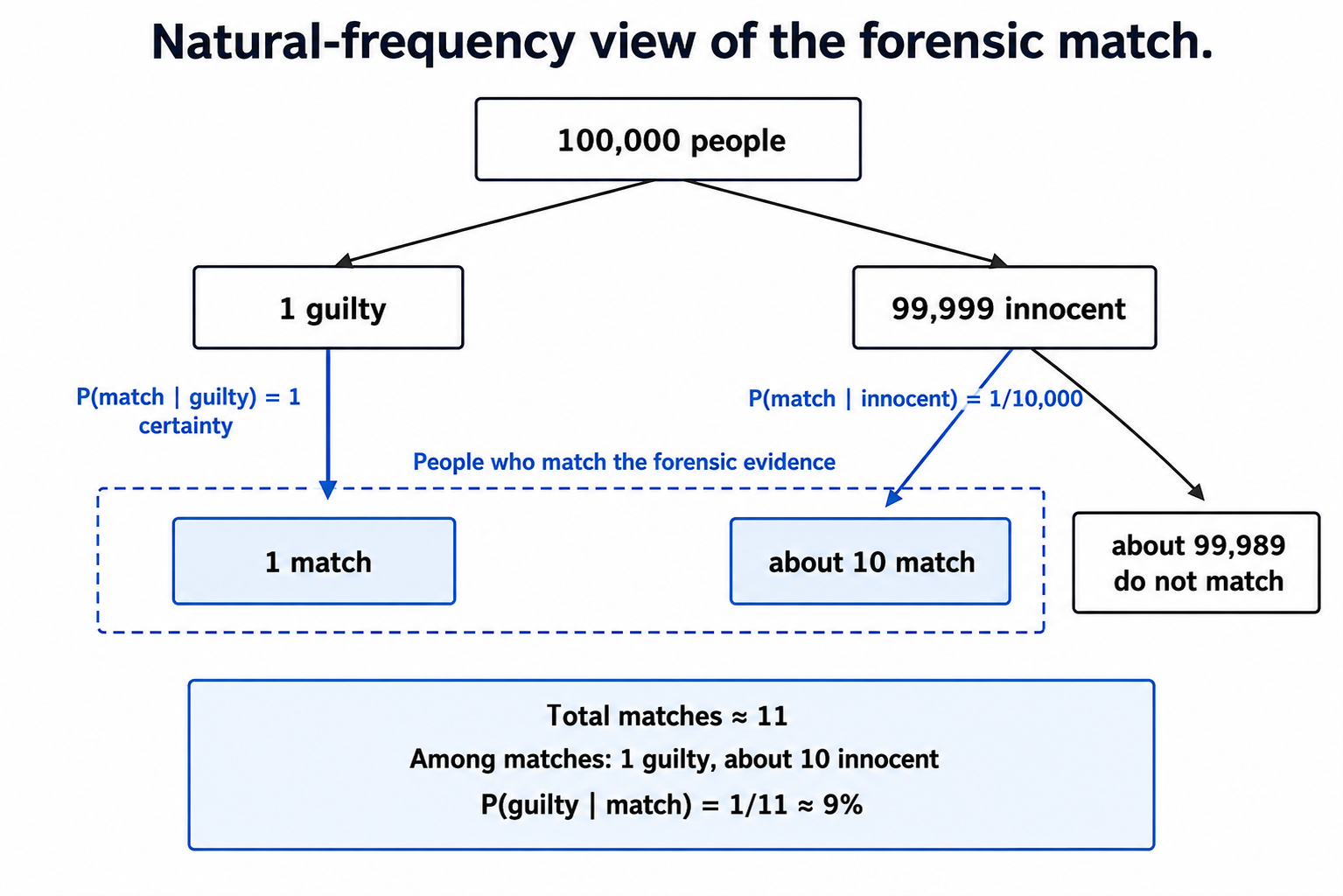
Before reaching for the formula, let's use the natural-frequency approach from earlier courses to build intuition. Out of the 100,000 people in the city:
1 is the actual guilty person, who will definitely match.
99,999 are innocent. Of these, roughly 99,999×0.0001≈10 will also match the forensic evidence purely by chance.
So about 11 people in the city would produce a match, and only 1 of them is guilty. If the defendant is simply one of those matches, the probability of guilt is:
P(guilty∣match)=111≈0.09
That is roughly a 9% chance of guilt — not the 99.99% the prosecutor implied. The "1 in 10,000" match rate sounded damning, but once we account for how many innocent people could also match, the picture changes dramatically.
We can confirm the counting result using the formula directly. Bayes' theorem gives us:
This matches our counting result: about 9%. The formula makes the role of the base rate explicit. Because P(guilty) is so tiny, even impressive-looking evidence cannot overcome it on its own. The base rate acts as an anchor, and no amount of ignoring it makes it go away.
Does this mean the forensic evidence is useless? Not at all. The match did shift the probability of guilt upward — from 0.001% to about 9%. In relative terms, that is a massive update, driven by a likelihood ratio of roughly 10,000. Just as we saw with spam cues in the last lesson, each piece of evidence moves the needle, but no single piece has to be the final word.
What the match does not establish is near-certain guilt by itself. It narrows the field from 100,000 people down to about 11, which is genuinely valuable investigative progress. But reaching a confident conclusion requires additional, independent evidence — witness testimony, motive, opportunity, or further forensic tests. Each of those further updates the posterior, just like adding more flagged words in the spam filter.
Here is a quick reference for distinguishing correct from incorrect claims:
Statement
Correct?
Why
"The chance an innocent person matches is 1 in 10,000."
✔
Correctly describes P(match∣innocent).
"There is only a 1 in 10,000 chance the defendant is innocent."
✘
Confuses P(match∣innocent) with P(innocent∣match).
"The match narrows the suspect pool but does not prove guilt alone."
✔
Evidence shifts belief but the conclusion depends on the base rate.
In this lesson, we examined the prosecutor's fallacy: the error of treating P(evidence∣innocence) as though it were P(innocence∣evidence). A "1 in 10,000" match probability turned out to correspond to only about a 9% probability of guilt once the base rate was properly included. The core lesson is the same one that runs through all of Bayesian reasoning: evidence does not speak for itself — it must always be weighed against the prior.
Now it is time to step into the courtroom yourself. In the practice exercises ahead, you will spot the fallacy in realistic arguments, compute how many innocent people would match, repair flawed reasoning by restoring the base rate, and explain in your own words what forensic evidence truly tells us.