Total Probability of Evidence
Introduction
Welcome back to Bayes' Theorem from the Ground Up! This is Lesson 4 of 5, so we are well into the home stretch of this course.
Over the last three lessons you have been assembling a toolkit piece by piece: counting with natural frequencies, writing down the Bayes' theorem formula, and identifying the prior, likelihood, and posterior inside any word problem. Today we focus on a quantity that ties all of those pieces together — the total probability of the evidence. This is the denominator in Bayes' theorem, and if you get it wrong, the entire posterior falls apart. By the end of this lesson, you will be able to compute the total probability of the evidence by summing every distinct path that could produce it, and you will understand why this sum is exactly what the denominator needs to be.
Every Piece of Evidence Has More Than One Source
Before we look at any formulas, let us build some intuition with an everyday situation. Imagine you hear a car alarm going off in a parking lot. That alarm (the evidence) could be triggered for more than one reason. Maybe someone actually tried to break into the car. Or maybe a loud truck rumbled past and set off the sensor. The alarm sounds the same either way.
This idea is at the heart of today's lesson. Whenever we observe a piece of evidence, we have to ask: What are all the different ways this evidence could have been produced? If we only count one way and ignore the others, our probability calculations will be off. A complete picture of the evidence requires every source, not just the one we happen to care about.
Two Paths That Produce the Same Evidence
In most Bayesian problems we work with two possible states of the world: the hypothesis is true, or the hypothesis is false. Each state offers its own path to producing the evidence we observed.
Let us revisit the circuit-board inspection scenario from Lesson 3. A board gets flagged by the camera. That flag could have arrived by either of two paths:
- True-positive path: The board genuinely has a defect, and the camera correctly caught it.
- False-positive path: The board is perfectly fine, but the camera mistakenly flagged it.
Both paths produce the exact same observation — a flagged board. To find the overall probability of seeing a flagged board, we need to account for both paths and add their contributions together. Leaving out either path would give us an incomplete, and therefore incorrect, total.
The Law of Total Probability
We can state this idea precisely using the quantities we already know how to identify. Recall from Lesson 3 that is the prior, is the likelihood when the hypothesis is true, and is the likelihood when the hypothesis is false. The total probability of the evidence combines both paths into a single expression:
Each term on the right side represents one complete path to the evidence:
- First term : Start with the chance the hypothesis is true, then multiply by how likely the evidence is when it is true.
- Second term : Start with the chance the hypothesis is false, then multiply by how likely the evidence is when it is not true.
Adding these two terms gives us every possible way the evidence can appear. Nothing is left out, and nothing is double-counted. That is why this formula is often called the law of total probability — it exhaustively covers all routes to the same observation.
Worked Example: Flagged Circuit Boards
Let us put this formula to work using the factory numbers from Lesson 3:
| Quantity | Value |
|---|---|
| Prior (5% of boards are defective) | |
| True-positive rate | |
| False-positive rate |
First, note that . Now we compute each path:
True-positive path:
False-positive path:
A probability tree makes these two contributions visible:
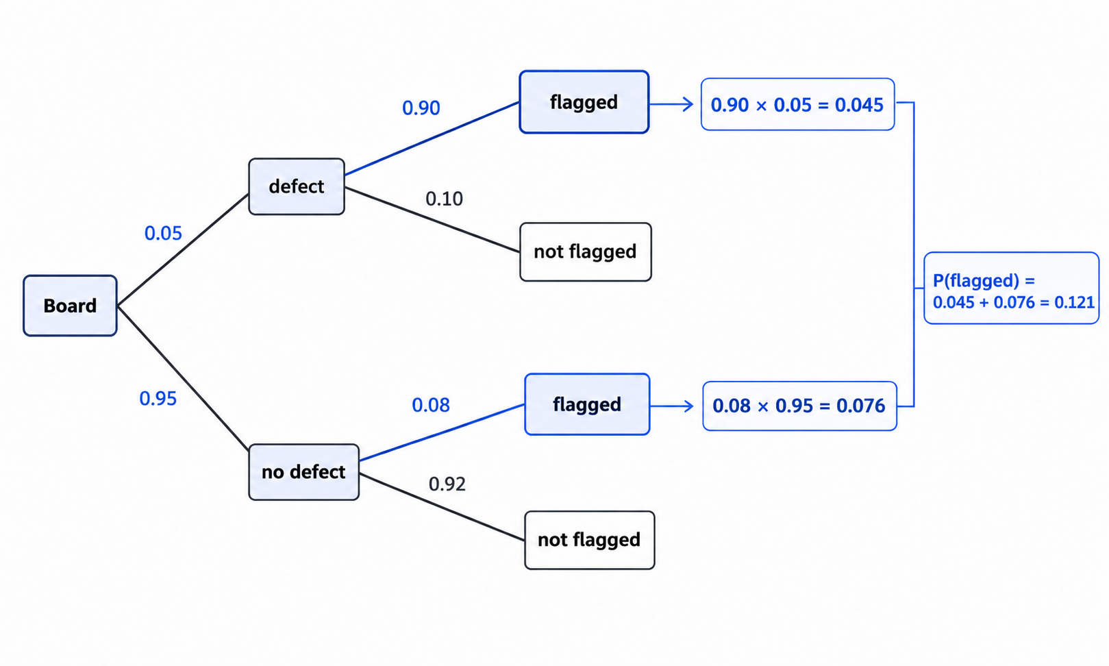
Adding both paths together:
So about 12.1% of all boards will be flagged by the camera. Notice something important: the false-positive path (0.076) actually contributes more to the total than the true-positive path (0.045). Even though the false-positive rate per board is low (8%), it applies to the much larger group of good boards (95% of all boards), so it adds up quickly.
Why This Is the Denominator
You may be wondering why the total probability of the evidence matters so much. The answer becomes clear when we look at the full Bayes' theorem formula:
The numerator, , is just the true-positive path — the portion of the evidence that is explained by the hypothesis being true. The denominator, , is the total amount of evidence from all paths combined.
Dividing one by the other gives us the fraction of the evidence that is actually due to the hypothesis. That fraction is the posterior. In our circuit-board example:
Only about 37.2% of flagged boards truly have a defect. Without the denominator, we would have no way to turn the numerator into a proper probability between 0 and 1. Think of the denominator as a scaling factor: it rescales the numerator so the result lands on the familiar probability scale.
When the False-Positive Path Dominates
The circuit-board example already hinted at this, but let us look at a more dramatic case. Suppose a streaming service uses an automated system to flag accounts suspected of subscription fraud.
| Quantity | Value |
|---|---|
| Only 0.5% of accounts are fraudulent | |
| The system catches 95% of fraudulent accounts | |
| The system falsely alerts on 3% of legitimate accounts |
Here . Let us compute each path:
True-positive path:
False-positive path:
Adding them:
The false-positive path (0.02985) is more than six times larger than the true-positive path (0.00475). Most alerts are coming from legitimate accounts, not from actual fraud. If we had ignored the false-positive path and used only the true-positive path as our denominator, we would have concluded that nearly every alert signals real fraud — a dangerously wrong answer. The total probability of the evidence corrects that mistake by including every route the alert could have taken.
Conclusion and Next Steps
In this lesson we learned that the probability of the evidence is built by summing every distinct path through which that evidence can occur. In a two-hypothesis setting, those paths are the true-positive path and the false-positive path. Together they form the denominator of Bayes' theorem, and this denominator ensures our posterior comes out as a valid, properly scaled probability. We also saw that the false-positive path can easily dominate when the hypothesis is rare, which is exactly why we must never leave it out.
Up next, you will practice computing the total probability of the evidence across several scenarios — including one where the false-positive path sneaks up on you. You will also explain in your own words why summing all paths produces the correct denominator, reinforcing the reasoning behind the formula.
