Reasoning with Natural Frequencies
Introduction
Welcome to Bayes' Theorem from the Ground Up, the second course in this learning path! In the previous course, we explored how probability can represent a degree of belief, how conditional probability filters our attention to relevant cases, and why is not the same as . We also learned that every belief starts with a base rate before any new evidence arrives.
Now it is time to put those ideas to work. In this first lesson, we will tackle a very common challenge: given some piece of evidence, how do we find the probability of a hypothesis? Rather than reaching for any formula, we will use a powerful technique called natural frequencies that turns percentages into simple whole-number counts we can reason about directly.
From Percentages to People
Imagine a doctor says: "This test catches 80% of true cases and has a 10% false alarm rate." Those percentages sound precise, but they can be surprisingly hard to combine in our heads. Which group does 80% apply to? Which group does 10% apply to? Mixing them up is one of the most common probability mistakes people make.
Here is a simpler approach: instead of juggling percentages, picture a concrete group of people and translate each percentage into a count of actual individuals. Suddenly, the math becomes nothing more than counting and dividing. This is the core idea behind natural frequencies, and it is exactly how we will solve inverse-probability problems in this lesson.
Setting Up an Imagined Population
The first step is to pick a convenient round number for our imagined population. A number like 1,000 works nicely because it makes percentage-to-count conversions easy.
Let's walk through a medical screening example. We begin with our base case—the information we have about the general population before we look at any specific test results:
- Base rate: 1% of the population has a rare disease.
- Detection rate: The test correctly identifies 80% of people who do have the disease.
- False alarm rate: The test incorrectly flags 10% of people who do not have the disease.
Now, imagine someone tests positive. What is the probability they actually have the disease? As we may recall from the previous course, this question is asking for , which is not the same as . Let's find it step by step.
Splitting by Hypothesis
We begin by dividing our 1,000 people into two groups based on who actually has the disease and who does not:
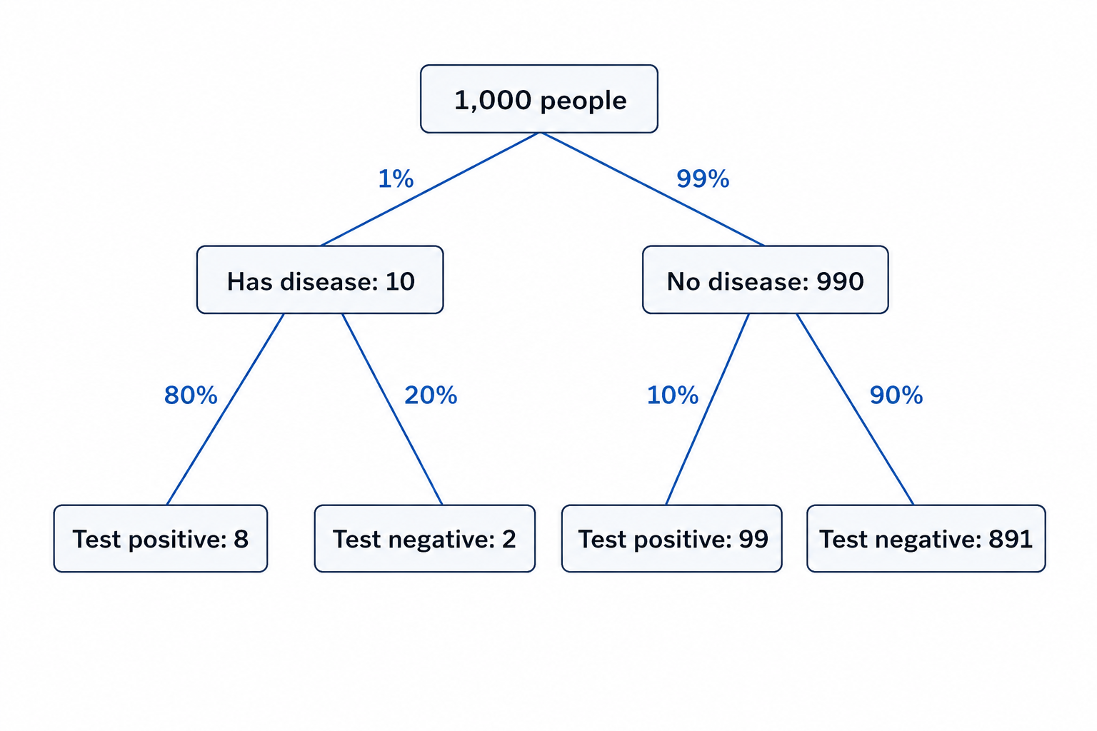
- Have the disease: 1% of 1,000 = 10 people
- Do not have the disease: the remaining 990 people
This is a direct application of the base rate. Notice that the healthy group is far larger, which is typical when a condition is rare. Keeping both groups visible from the start prevents us from losing sight of just how many people could generate false alarms.
Sorting by Evidence
Next, we apply the test to each group separately.
For the 10 people who have the disease, the test catches 80% of them:
For the 990 people who do not have the disease, the test falsely flags 10% of them:
A split diagram makes the counting structure visible:
We can now place everyone into a tidy count table:
| Test Positive | Test Negative | Total | |
|---|---|---|---|
| Has disease | 8 | 2 | 10 |
| No disease | 99 | 891 | 990 |
| Total | 107 | 893 | 1,000 |
Every person in our imagined population is accounted for, and we can verify this by checking that every row and column adds up correctly.
Reading the Answer from the Counts
Our question was: "Given a positive test, what is the probability the person actually has the disease?" To answer it, we look at everyone who tested positive. That is the 107 people in the "Test Positive" column. Of those 107, only 8 actually have the disease. So:
That is roughly 7.5%. Even though the test sounds quite accurate, a person who tests positive still has less than an 8% chance of truly having the disease. The reason is that the disease is so rare: the 99 false alarms from the large healthy group vastly outnumber the 8 true catches from the small sick group.
This result often surprises people, and that surprise is exactly why natural frequencies are so valuable. By laying out the counts, we can see where the numbers come from instead of relying on gut instinct.
The General Recipe
The medical example above illustrates a method we can apply to any inverse-probability problem. Here is the recipe:
- Pick a population size (such as 1,000 or 10,000) that keeps the arithmetic clean.
- Split by hypothesis: use the base rate to divide the population into a hypothesis-true group and a hypothesis-false group.
- Split by evidence: apply the relevant rates to each group to find how many people in each group produce the evidence.
- Read the answer: divide the hypothesis-true-and-evidence count by the total evidence count.
In general terms:
No advanced formula is needed. The whole-number counts make the relationships visible and keep us from accidentally swapping the two directions of a conditional.
Conclusion and Next Steps
In this lesson, we learned how to solve inverse-probability problems by translating percentages into whole-number counts across an imagined population. By splitting people first by hypothesis and then by evidence, we can read the answer directly from a simple count table. This technique, known as reasoning with natural frequencies, turns a tricky probability question into straightforward counting.
In the next lesson, we will see how this same logic can be captured in a compact formula called Bayes' theorem. But first, let's put natural frequencies into practice with the exercises ahead, where we will build count breakdowns and extract answers step by step.
