Bayes Theorem Formula
Introduction
Welcome back to Bayes' Theorem from the Ground Up! In the first lesson of this course, we solved an inverse-probability problem entirely by counting. We imagined a population, split it into groups, and read the answer straight from a table of whole numbers. That natural-frequency approach is intuitive, and it works every time.
In this second lesson, we will take that counting logic and compress it into a single mathematical expression: Bayes' theorem. By the end, we will be able to write the formula, name every piece in it, and explain exactly how each symbol maps back to the natural-frequency reasoning we already know. The formula will not replace the counting method; it will simply let us skip the step of choosing an imaginary population.
From a Table to a Single Line
Recall that every natural-frequency solution we built in the previous lesson followed the same pattern: divide the population by hypothesis, apply rates to get evidence counts, then read the answer as a fraction. No matter which numbers we used, the final step always looked like this:
That fraction is the heart of everything we did. A formula simply replaces the concrete counts with the rates that produced them, so we no longer need to pick a population size or fill in a table. Think of the formula as a shortcut that packages all four steps of our counting recipe into one compact line.
From Counts to Rates
Let's trace how the population cancels out. In our medical screening example, we started with 1,000 people and found:
Those counts came directly from the original rates:
- 8 true positives =
- 99 false positives =
- 107 total positives =
Every term begins with the population size 1,000. If we divide both the numerator and the denominator by 1,000, it drops out entirely:
We are left with nothing but the original rates. The population was just scaffolding; the formula keeps only what matters. This is the key insight: the imaginary population helps us think, but mathematically it always cancels, leaving behind the rates we started with.
The Formula
Using standard notation, Bayes' theorem says:
Here, stands for the hypothesis and stands for the evidence. The symbol means "not ," the scenario where the hypothesis is false. Since the hypothesis must be either true or false, it is always the case that .
In plain language: the probability of the hypothesis given the evidence equals the cases where both the hypothesis and the evidence hold, divided by all the cases where the evidence holds. That is the exact same sentence we used when reading answers from our count table — nothing new, just a more compact way to say it.
A quick tree view shows exactly how the numerator and denominator fit together:
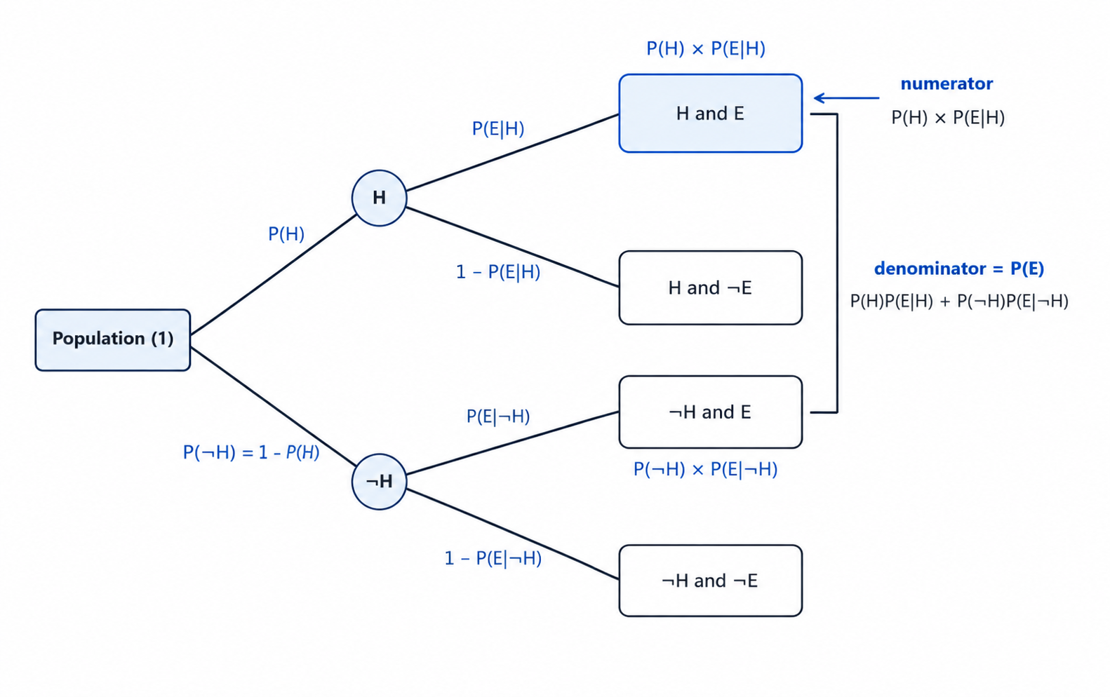
The top branch gives us the numerator, and both branches together give us the denominator.
Mapping Each Term
Each piece of the formula lines up with a step from our natural-frequency recipe. The table below makes the connection explicit:
| Symbol | Name | Counting Meaning |
|---|---|---|
| Prior | Fraction of the population where the hypothesis is true (the base rate) | |
| Likelihood | Fraction of the hypothesis-true group that shows the evidence | |
| Prior for the alternative | Fraction of the population where the hypothesis is false, i.e. | |
| Likelihood under the alternative | Fraction of the hypothesis-false group that still shows the evidence, often a false-alarm rate in screening examples | |
| Posterior | Fraction of all evidence cases that belong to the hypothesis-true group |
The numerator, , gives the proportion of the whole population that is both hypothesis-true and evidence-present. In our medical example, that was , corresponding to 8 out of every 1,000 people.
The denominator adds up every way the evidence can appear. It combines the hypothesis-true path and the hypothesis-false path into one total. This is the same "Total Positive" column we read from our count table, just expressed as a proportion rather than a raw count.
Verifying with the Medical Example
Let's confirm that the formula reproduces the answer we found by counting. We plug in the same rates we used in the previous lesson:
- ,
- ,
Substituting into the formula:
That is the same 7.5% we obtained from the count table. The formula did not change the reasoning; it simply expressed it without the imaginary population. Any time we feel unsure about the formula, we can always go back to counting — both routes lead to the same destination.
The Shorter Form
You will sometimes see Bayes' theorem written more compactly:
Here, stands for the total probability of the evidence, which is just the entire denominator we already computed. It captures "all the cases where the evidence holds" in a single symbol. We will practice computing step by step in a later lesson devoted to that denominator. For now, the key point is that is the sum of every path that produces the evidence — exactly what the bottom row of our frequency table showed.
Both forms of the theorem say the same thing. The expanded version spells out exactly how is built, while the shorter version tucks that work behind a single symbol. Use whichever form makes the current problem easier to follow.
Conclusion and Next Steps
In this lesson, we translated the natural-frequency counting method into Bayes' theorem. The formula is not a new kind of reasoning; it is the same "hypothesis-and-evidence cases divided by all evidence cases" logic written in compact notation. The prior sets the base-rate split, the likelihood and false-alarm rate sort each group by evidence, and the denominator totals every path to the evidence.
Now it is time to make these connections second nature. In the practice exercises ahead, you will match each symbol to its counting meaning, fill in missing pieces of the formula, and explain in your own words why Bayes' theorem is simply the frequency method captured in a single line. Once those connections feel solid, we will move on to the next lesson, where we focus on confidently identifying the prior, likelihood, and posterior in real-world scenarios — even when the wording tries to trip us up.
