Welcome to 2D Grids and Matrix Math. In this first lesson, we’ll take the next step beyond 1D array indexing and start thinking in rows and columns. The goal is practical: each CUDA thread will compute which matrix element it owns, then convert that 2D position into the correct location inside a linear memory buffer.
The Power of Matrix Operations
Up to this point, you may have primarily seen CUDA used for 1D operations, like adding two arrays. While 1D processing is a great way to learn the basics of parallel threads, real-world GPU workloads often revolve around linear algebra and matrix operations.
Matrices are the building blocks behind many of the most important areas in modern computing:
Machine Learning & LLMs: Training and inference for models like GPT rely on massive matrix multiplies.
Gaming & Graphics: Pixels and vertices are processed through coordinate transforms and shader math.
Scientific Simulations: Weather, fluid dynamics, and physics simulations operate on grid-shaped data.
To work efficiently with data like this, we want to launch threads in a way that matches the problem’s shape.
Why Matrices Push Us Toward 2D Thinking
A matrix isn’t just a long list of values. It has:
a width (columns)
a height (rows)
So each thread should ideally know two things:
which column it belongs to
which row it belongs to
This 2D way of thinking becomes especially important for matrix multiplication, image processing, stencil updates, and many other kernels where neighbors and tiles matter.
From 1D Launches to dim3
So far, we have mostly launched kernels in a way that looks 1D:
int threadsPerBlock = 256;
That’s perfectly valid, but under the hood CUDA launch dimensions are represented by a type called dim3, which has three components:
.x
.y
.z
So the launch above is effectively the same as:
dim3 threadsPerBlock(256, 1, 1);
The unused dimensions are not hiding extra threads—they simply default to 1.
The same idea applies to blocks inside the grid. Blocks live inside a grid, and that name is literal: the launch shape can be arranged like a grid. Up to now, we’ve used a 1D grid, so we only needed .x.
That’s why earlier 1D kernels used indexing like this:
int id = blockIdx.x * blockDim.x + threadIdx.x;
This works for flat arrays. But for matrices, it’s much more natural to use two axes:
.x for columns
.y for rows
Preparing Memory and the Launch Shape
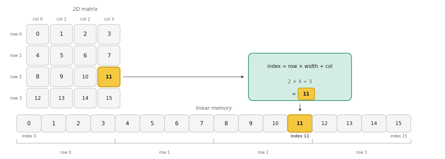
From 2D Coordinates to 1D Memory
Don’t Confuse the CUDA Grid with the Matrix
Defining the Kernel
Now we can define the kernel itself. Each thread computes its global column and row, checks whether it’s inside the matrix, then writes to the correct linear position.
__global__ void matrixInit(float* matrix, int width, int height) { int col = blockIdx.x * blockDim.x + threadIdx.x; int row = blockIdx.y * blockDim.y + threadIdx.y; if (col < width && row < height) { int index = row * width + col; matrix[index] = static_cast<float>(index); }}
The indexing lines are the key:
blockIdx.x and threadIdx.x locate the thread across the grid (columns)
blockIdx.y and threadIdx.y locate the thread down the grid (rows)
Together, they produce a global matrix coordinate.
The if check matters because the rounded-up grid may launch threads that fall outside the valid matrix area. Inside bounds, each thread stores its own linear index, which makes the mapping easy to verify.
Launching the Kernel and Validating Data
With memory ready, the launch shape chosen, and the kernel defined, we can run it. After the launch, we check for launch errors, wait for the GPU to finish, copy the results back, and verify that every element matches the expected linear index.
    matrixInit<<<numBlocks, threadsPerBlock>>>(d_matrix, W, H);
    CUDA_CHECK(cudaGetLastError());
    CUDA_CHECK(cudaDeviceSynchronize());

    CUDA_CHECK(cudaMemcpy(h_matrix.data(), d_matrix, bytes, cudaMemcpyDeviceToHost));

    bool success = true;
    for (int i = 0; i < W * H; ++i) {
        if (h_matrix[i] != static_cast<float>(i)) {
            success = false;
            break;
        }
    }
A CUDA kernel launch is asynchronous, so cudaDeviceSynchronize() ensures the kernel has finished before we inspect results.
The validation loop is a simple but effective test: if our 2D-to-1D mapping is correct, element i should contain exactly i.
Printing the Matrix and Final Cleanup
Finally, we print the data in matrix form, report whether the indexing worked, then release device memory and return a success code. The nested loops rebuild the 2D view on the host using the same row-major formula i * W + j.
Reading across each row, we see the expected linear order from 0 to 11, confirming that each thread wrote to the correct element.
Conclusion and Next Steps
In this lesson, we expanded our view of CUDA launches from 1D to 2D using dim3. We prepared a 2D launch, computed global row and col values, converted them to a linear index using row * width + col, and verified that every matrix element landed in the correct place.
This pattern is foundational in CUDA because many GPU problems involve images, matrices, and other grid-shaped data. In the practice section ahead, you’ll reinforce this idea by writing and checking 2D indexing yourself.
Even though a matrix looks two-dimensional, in memory it is typically stored as one long linear buffer. That means every thread must do two jobs:
compute its 2D matrix position
convert that position into a single linear index
For a matrix stored in row-major order, the mapping is:
index=row×width+col
This is the pattern we’ll use throughout the lesson:
Compute col
Compute row
Convert them into index
This is the bridge between CUDA’s 2D thread layout and the actual memory buffer on the GPU.
Note: The figure below illustrates this mapping for a 4×4 matrix (W=4,H=4), whereas our code example uses a 4×3 matrix.
Even if you launch with a “2D” dim3, the CUDA execution configuration is just a way of organizing threads—it does not magically turn your data into a real 2D matrix type.
The good news is that the grid, blocks, and threads really are multidimensional (depending on the dim3 values you choose). CUDA abstracts that for you by providing blockIdx.{x,y,z} and threadIdx.{x,y,z} so you don’t have to manually “flatten” thread IDs yourself.
Inside the kernel, however, your matrix is still just a float* pointing to a flat 1D buffer in linear memory. That means you still explicitly compute (col, row) from those multidimensional thread coordinates, and then convert that 2D position into a single linear index.
This distinction matters because memory layout (like row-major vs column-major) determines the correct mapping formula, not the launch shape. In other words, dim3 makes it easy to think in 2D for threads, but you are responsible for mapping that to the correct address in memory.
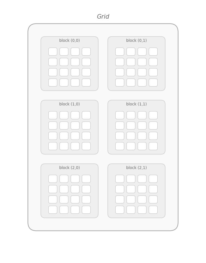
Note: The figure below demonstrates a 2×3 grid of 4×4 blocks. This configuration is different from our code's 4×3 matrix and 2×2 blocks, but it highlights how the grid organizes threads.
Before we define the kernel, we choose a matrix size, allocate memory, and decide how threads should be arranged.
C++
int main() {
    const int W = 4, H = 3;
    const size_t bytes = W * H * sizeof(float);

    std::vector<float> h_matrix(W * H, -1.0f);
    float* d_matrix = nullptr;

    CUDA_CHECK(cudaMalloc(&d_matrix, bytes));

    dim3 threadsPerBlock(2, 2);
    dim3 numBlocks((W + threadsPerBlock.x - 1) / threadsPerBlock.x,
                   (H + threadsPerBlock.y - 1) / threadsPerBlock.y);
For this example:
W = 4 means 4 columns
H = 3 means 3 rows
total elements = W * H = 12
On the host, we store the matrix in a std::vector. On the device, we allocate a raw pointer with cudaMalloc.
The important new idea is the 2D block shape:
C++
dim3 threadsPerBlock(2, 2);
Instead of a flat 1D block, each block is now a small 2 x 2 tile of threads. We chose (2, 2) here specifically to fit our tiny 4×3 matrix and demonstrate how multiple blocks are created. In professional CUDA code, you will typically see larger block sizes—such as 16 x 16 or 32 x 32—to better utilize the GPU hardware and align with warps (groups of 32 threads).
Next, we compute how many blocks we need in each direction:
This “round up” division ensures the grid is large enough even if the matrix dimensions don’t divide evenly by the block dimensions. The tradeoff is that we may launch a few extra threads, which is why we’ll do a bounds check inside the kernel.