Welcome to the second lesson of "Training Neural Networks: The Backpropagation Algorithm"! In our previous lesson, we introduced the concept of loss functions and focused specifically on mean squared error (MSE) as a way to measure how far our neural network's predictions deviate from the ground truth.
We learned that a loss function acts as a report card for our model's performance, with lower values indicating better predictions. But a critical question remains: how do we actually use this loss function to improve our model? This is where gradient descent comes in.
Gradient descent is the fundamental optimization algorithm that powers most neural network training. It provides a systematic way to adjust the model's weights to minimize the loss function. Today, we'll build an intuitive understanding of this powerful algorithm and implement a simple example to see it in action.
Understanding Optimization Landscapes
Let's start by considering the broader optimization problem we're trying to solve when training neural networks.
When training a neural network, our goal is to find the set of weights that minimize the loss function. We can visualize this as finding the lowest point in a landscape where:
The landscape represents our loss function.
The coordinates on this landscape represent our model parameters (weights).
The height at each point represents the loss value.
Our objective is to find the lowest point (global minimum) in this landscape.
For simple problems, we could try to solve this mathematically by setting the derivative of the loss function with respect to each weight to zero and solving the resulting equations. However, for neural networks with thousands or millions of parameters, this approach is computationally impossible.
Instead, we need an iterative algorithm that can gradually move toward the minimum. This is precisely what gradient descent does — it starts at some point on the loss landscape and takes steps in the direction that leads downhill most quickly.
Visualizing a Loss Landscape
Gradient Descent: The Intuition
A Simple 1D Illustration of Gradient Descent
The Role of Learning Rate
The learning rate is one of the most critical hyperparameters in neural network training. It determines how large a step we take in the direction of the negative gradient. Think of it as controlling your stride length:
A large learning rate means taking big steps, which can help you move faster but might cause you to overshoot the minimum or even diverge.
A small learning rate means taking small, cautious steps, which gives more precise movement but might take much longer to reach the minimum.
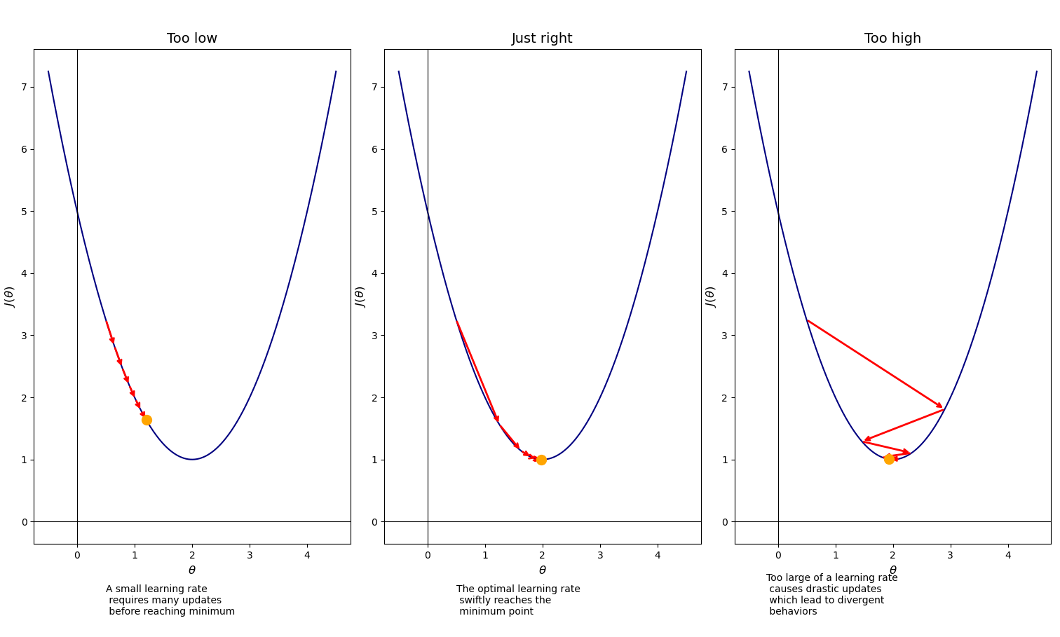
Let's visualize what happens with different learning rate choices:
Left: A learning rate that's too low (0.05) makes tiny steps, requiring many iterations to reach the minimum. Middle: An appropriate learning rate (0.25) converges efficiently in just a few steps. Right: A learning rate that's too high (0.8) causes the algorithm to overshoot and oscillate wildly, potentially diverging.
Choosing an appropriate learning rate is a delicate balance. Typically, values between 0.1 and 0.0001 are common starting points, but the optimal learning rate varies greatly depending on the specific problem, network architecture, and dataset. In advanced training scenarios, techniques like learning rate schedules and adaptive learning rates have been developed to automatically adjust this crucial parameter during training.
Implementing 1D Gradient Descent: The Setup
Implementing 1D Gradient Descent: The Algorithm
Now, let's implement the gradient descent algorithm to find this minimum:
current_x <- 0.0 # Initial guesslearning_rate <- 0.1epochs <- 30cat(sprintf("Minimizing f(x) = x^2 - 4x + 5. Starting at x = %.2f\n", current_x))for (i in 1:epochs) { # Calculate the gradient at the current position gradient <- derivative_simple_quadratic(current_x) # Update the position by moving in the opposite direction of the gradient current_x <- current_x - learning_rate * gradient # Calculate the new function value loss <- simple_quadratic_function(current_x) # Print progress at specified intervals if (i %% 5 == 0 || i == 1) { # Print every 5 epochs or the first one cat(sprintf("Epoch %2d: x = %6.3f, f(x) = %6.3f, gradient = %6.3f\n", i, current_x, loss, gradient)) }}
Let's break down what's happening in this implementation:
We start at an initial position (x=0) — this is like placing ourselves randomly on the hill.
For each epoch (iteration):
Calculate the gradient (slope) at our current position.
Update our position by moving in the opposite direction of the gradient, scaled by the learning rate.
Calculate the new function value (loss) to track our progress.
Print our status at regular intervals to visualize the optimization journey.
This simple loop captures the essence of gradient descent, whether in 1D or in the much higher-dimensional space of neural network weights.
Visualizing the Optimization Journey
When we run our gradient descent implementation, we see the following output:
Minimizing f(x) = x^2 - 4x + 5. Starting at x = 0.00Epoch 1: x = 0.400, f(x) = 3.560, gradient = -4.000Epoch 5: x = 1.345, f(x) = 1.429, gradient = -1.638Epoch 10: x = 1.785, f(x) = 1.046, gradient = -0.537Epoch 15: x = 1.930, f(x) = 1.005, gradient = -0.176Epoch 20: x = 1.977, f(x) = 1.001, gradient = -0.058Epoch 25: x = 1.992, f(x) = 1.000, gradient = -0.019Epoch 30: x = 1.998, f(x) = 1.000, gradient = -0.006After 30 epochs, estimated minimum x = 1.998, f(x) = 1.000The true minimum is at x = 2.0, f(x) = 1.0
This output reveals several important patterns about how gradient descent works:
We start at x=0 with a steep negative gradient (-4.000), indicating we should move to the right.
In the first update, we jump to x=0.400 (0 - 0.1 * (-4)).
As we continue making updates, the size of each step gets smaller as the gradient approaches zero.
By epoch 30, we've reached x=1.998, extremely close to the true minimum at x=2.0.
Notice how the gradient approaches zero as we get closer to the minimum.
We can observe key characteristics of gradient descent:
Convergence pattern: Our progress is rapid at first and then slows as we approach the minimum.
Gradient magnitude: The gradient naturally gets smaller as we get closer to the minimum.
Approximation: We get very close to, but not exactly at, the true minimum with a finite number of iterations.
This pattern of rapid initial progress followed by slower refinement is characteristic of gradient descent and will be similar when training neural networks with millions of parameters.
Gradient Descent in Neural Networks
Now that we understand gradient descent in a simple 1D context, let's extend this intuition to neural networks.
In a neural network:
Instead of a single variable x, we have thousands or millions of weights.
The loss function is much more complex than our simple quadratic.
The landscape has many dimensions and might include multiple local minima and saddle points (flat regions where the gradient is near zero but we haven't reached a minimum), making optimization more challenging.
The principle remains the same: calculate the gradient of the loss with respect to each weight and update weights in the opposite direction of the gradient.
The update rule for a single weight in a neural network looks like:
While our 1D example directly computed the gradient as 2x-4, calculating gradients in neural networks is more complex, requiring a technique called backpropagation (which we'll cover in upcoming lessons).
The key insight is that regardless of the dimensionality or complexity, gradient descent follows the same fundamental principle: iteratively update parameters by moving in the direction that reduces the loss function most rapidly. It's this elegant simplicity that makes gradient descent such a powerful algorithm for neural network training.
Conclusion and Next Steps
Congratulations on mastering gradient descent, the fundamental optimization algorithm behind neural network training! You've learned the intuitive concept of "following the slope downhill," understood how the learning rate affects convergence, implemented a 1D example, and discovered how these principles extend to neural networks. This algorithm forms the backbone of the learning process, allowing networks to systematically improve their predictions by minimizing the loss function.
In the upcoming practice exercises, you'll gain hands-on experience with gradient descent and explore how different parameters affect the optimization process. After solidifying these concepts through practice, we'll advance to the backpropagation algorithm, which efficiently calculates the gradients needed for training multi-layer neural networks.
Be a part of our community of 1M+ users who develop and demonstrate their skills on CodeSignal
R
current_x <- 0.0 # Initial guesslearning_rate <- 0.1epochs <- 30cat(sprintf("Minimizing f(x) = x^2 - 4x + 5. Starting at x = %.2f\n", current_x))for (i in 1:epochs) { # Calculate the gradient at the current position gradient <- derivative_simple_quadratic(current_x) # Update the position by moving in the opposite direction of the gradient current_x <- current_x - learning_rate * gradient # Calculate the new function value loss <- simple_quadratic_function(current_x) # Print progress at specified intervals if (i %% 5 == 0 || i == 1) { # Print every 5 epochs or the first one cat(sprintf("Epoch %2d: x = %6.3f, f(x) = %6.3f, gradient = %6.3f\n", i, current_x, loss, gradient)) }}
text
Minimizing f(x) = x^2 - 4x + 5. Starting at x = 0.00Epoch 1: x = 0.400, f(x) = 3.560, gradient = -4.000Epoch 5: x = 1.345, f(x) = 1.429, gradient = -1.638Epoch 10: x = 1.785, f(x) = 1.046, gradient = -0.537Epoch 15: x = 1.930, f(x) = 1.005, gradient = -0.176Epoch 20: x = 1.977, f(x) = 1.001, gradient = -0.058Epoch 25: x = 1.992, f(x) = 1.000, gradient = -0.019Epoch 30: x = 1.998, f(x) = 1.000, gradient = -0.006After 30 epochs, estimated minimum x = 1.998, f(x) = 1.000The true minimum is at x = 2.0, f(x) = 1.0
Let's see a visual example of how a loss landscape may look for a sample quadratic function that depends on two weights, w1 and w2:
Left (3D view): Here you can see the "bowl-shaped" surface of our loss. The height represents the loss value for each (w1,w2) pair. The red dot marks the global minimum at (2,3), where the loss is zero.
Right (contour view): This top-down plot shows lines of equal loss (contours). Each ring corresponds to a higher or lower loss level. Darker (inner) regions are lower loss, and the red dot again highlights the minimum.
To make our intuition even clearer, let's look at a concrete 1D example. Below is a plot of the same quadratic function we'll implement in code, f(x)=x2−4x+5, along with a few sample points showing the direction and magnitude of the gradient at each step:
The blue curve shows our loss landscape in one dimension. You can see it dips down to its global minimum at x=2, where f(2)=1.
Orange dots mark several starting positions along the curve. At each of these points, we compute the derivative (gradient) of the function.
Black arrows indicate the direction and relative size of each update step:
Longer arrows mean a steeper slope (larger gradient) and thus a bigger move.
Shorter arrows mean we're getting closer to the bottom, so the slope is smaller and our steps shrink naturally.
Watching these arrows point "downhill" toward the minimum captures exactly how gradient descent navigates the landscape — taking bigger strides when the slope is steep and slowing down as it approaches the lowest point. In our upcoming code example, you'll see this same pattern emerge numerically, just as you see it here visually.
The core idea behind gradient descent is surprisingly intuitive: follow the slope downhill.
Imagine you're standing on a hill in dense fog and want to reach the bottom. Without being able to see the entire landscape, a sensible strategy would be to:
Feel the ground around you to determine which direction is steepest downhill.
Take a step in that direction.
Repeat until you reach a point where you can't go any lower.
This is exactly how gradient descent works:
The gradient is the mathematical equivalent of feeling the ground around you — it tells you the direction of steepest ascent.
By moving in the negative direction of the gradient, you move in the direction of steepest descent.
The size of your step is determined by a parameter called the learning rate.
Mathematically, if we have a scalar-valued function f(x1,x2,…,xn) that depends on n variables, the gradient of f is the vector of partial derivatives:
∇f(x1,x2,…,xn)=[∂x1∂f,∂x2∂f,…,∂xn∂f]
This gradient vector points in the direction of steepest increase of the function. Each component tells us how much the function changes when we move slightly in the direction of that particular variable. In our neural network context, each xi represents a weight, and the gradient tells us how the loss changes with respect to each weight.
We can express a single update step of gradient descent as:
Where the gradient is the derivative of the function with respect to the position. This simple update rule forms the foundation of neural network optimization, despite the impressive complexity of modern networks.
To build intuition, let's implement gradient descent to find the minimum of a simple one-dimensional function. We'll use a quadratic function as our example: