You have now met every moving part of a three-variable solve, but always one at a time. Someone else picked the target variable, or handed you the reduced system, or told you which equation to check. Welcome to the fifth lesson of Three-Variable Systems and a First Look Beyond, where that scaffolding comes down.
From here on, the input is a bare system of three equations and the output is a verified ordered triple, with every decision in between left to you. The individual moves will feel familiar. What is new is the coordination — deciding the route before you drive it, and keeping a fifteen-line solve honest from the first line to the last.
The Whole Pipeline at a Glance
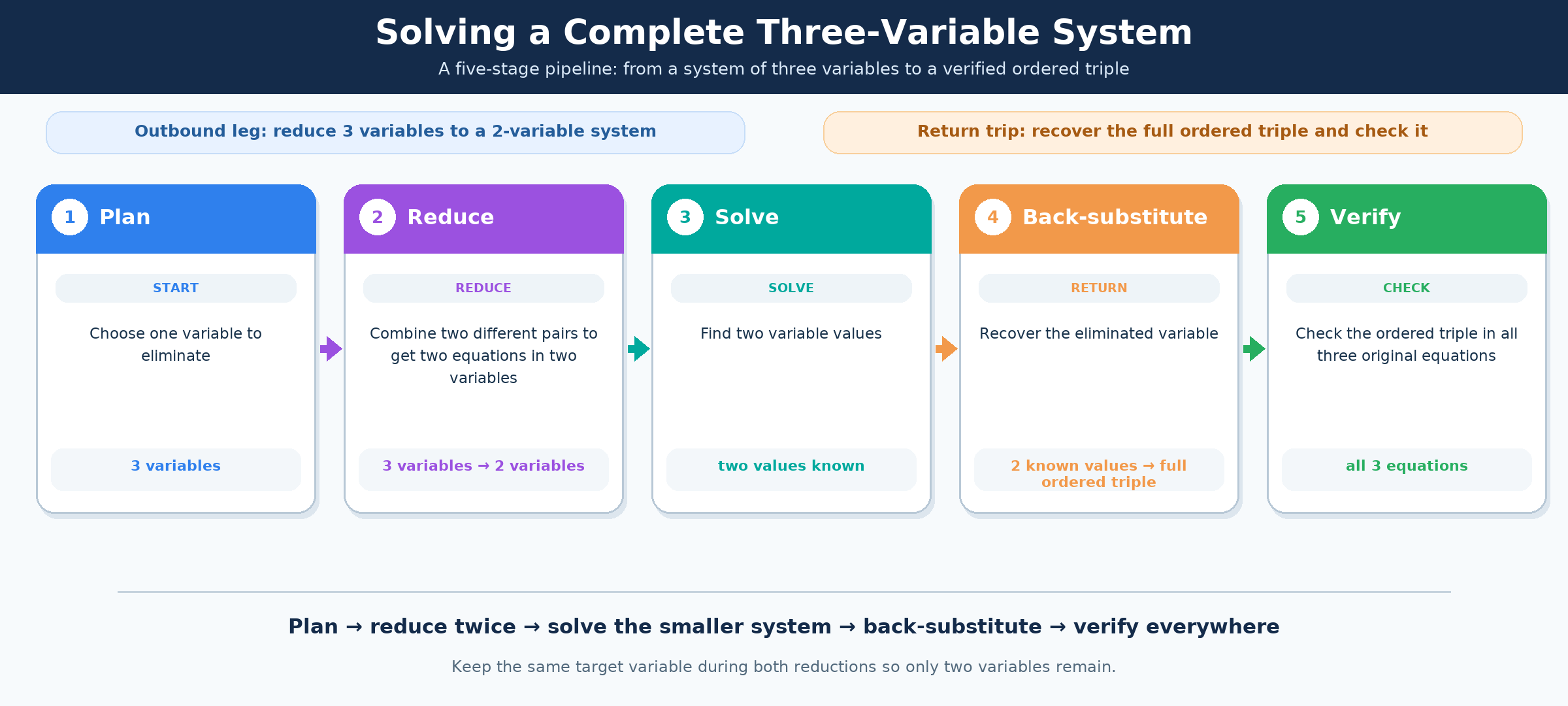
A complete solve is a fixed sequence, and knowing that sequence by heart is half the battle. No matter how friendly or ugly the numbers are, we travel the same five stages:
Plan. Pick the variable to eliminate first, and note which pairs of equations to combine.
Reduce. Eliminate that variable from two different pairs, scaling where needed, to get a two-variable system.
Solve. Handle the reduced system with substitution or elimination, whichever is cheaper.
Back-substitute. Return to an original equation to recover the eliminated variable.
Verify. Test the full triple in all three original equations.
As you may recall from the previous lesson, stages 1 and 2 are the outbound leg — three unknowns collapsing into two — and stages 3 through 5 are the return trip. Any of the three variables can serve as the target, and every valid choice leads to the same triple; the choice only changes how much arithmetic you sign up for. That is exactly why stage 1, the one step we have never practiced deliberately, is where we begin.
Planning Before Computing
Before writing a single line, read the system down the columns rather than across the rows. Each column holds one variable's three coefficients, and the shape of that column tells you what eliminating it will cost: a column of 1s and −1s means straight addition or subtraction, while a column of unrelated numbers means scaling both equations in a pair.
Take this system as an example:
⎩⎨⎧(1)x+y+z=6(2)x−y+2z=5(3)2x+y−z=1
Variable
Coefficients
Cost to eliminate
x
1,1,2
One subtraction, one scaling
y
1,−1,1
Pure addition, no scaling
z
1,2,−1
Two scalings
The y column decides it for us: the opposite signs mean we can add equations as they stand. Thirty seconds of planning here saves several lines of arithmetic — and several chances to slip — later on.
Join the 1M+ learners on CodeSignal
Be a part of our community of 1M+ users who develop and demonstrate their skills on CodeSignal
A Full Solve with No Scaling
Reducing a System That Needs Scaling
Finishing the Harder Solve
From Receipts to a Triple
Habits That Keep a Long Solve on Track
Conclusion and Next Steps
In this lesson we drove the complete route twice: read the columns to choose a target, reduce with two pairwise combinations, solve the reduced two-variable system, back-substitute into a convenient original equation, and verify the triple everywhere. The first system cancelled for free, the second demanded scaling at two separate stages, and both finished with an answer we could actually defend.
Now the route is yours to drive. In the practice ahead you will plan a solve before touching any arithmetic, trace a pipeline stage by stage, solve two complete systems of increasing difficulty, and finally recover three café prices from three receipts. Every piece is already in your hands — this is where they click together.
Following the plan, we eliminate y from two different pairs. Equations (1) and (2) add cleanly, and so do (2) and (3):
(1)+(2):(2)+(3):2x+3z=113x+z=6
Both results involve only x and z, so the reduction is finished and stage 3 begins. In the second equation z has coefficient 1, so multiplying that equation by 3 gives 9x+3z=18; subtracting 2x+3z=11 leaves 7x=7, so x=1, and 3(1)+z=6 gives z=3.
Now we return to an original equation for the variable we discarded. Equation (1) carries a coefficient of 1 on y, making it the friendliest landing spot: 1+y+3=6, hence y=2. The candidate is (1,2,3) — written in (x,y,z) order, not the order the values appeared — and it survives all three checks:
(1):(2):(3):1+2+3=6✓1−2+2(3)=5✓2(1)+2−3=1✓
Most systems are not that polite. Nothing cancels on sight in this one:
⎩⎨⎧(1)2x+3y+z=1(2)4x−y+5z=19(3)3x+2y−4z=1
When no column cancels for free, the planning question shifts from "which column cancels?" to "which column needs the smallest multipliers?" The y column is 3,−1,2, and that lone −1 in equation (2) means each pair needs only one equation scaled, using multipliers of 3 and 2. The z column, by contrast, would require multipliers of 5 and 4, so y is the cheaper target.
Notice that every term of the first result shares a factor of 2, so dividing through turns it into 7x+8z=29. Tidying a reduced equation the moment it appears costs one glance and keeps the next stage light.
Our reduced system is
{7x+8z=2911x+6z=39
Neither variable is isolated and neither would isolate without fractions, so elimination beats substitution here. Multiplying the first equation by 3 and the second by 4 matches both z terms at 24z:
−21x+24z=8744x+24z=156−23x=−69
That gives x=3, and 7(3)+8z=29 becomes 8z=8, so z=1. For the third value we go back to equation (2), where y has coefficient −1:
4(3)−y+5(1)=19
This simplifies to 17−y=19, so −y=2 and y=−2. Verifying (3,−2,1) in all three originals:
Two systems, two very different levels of arithmetic, one identical route from start to finish.
Systems like these appear whenever three unknown quantities hide inside several totals. Picture a café where three coworkers order combinations of coffee, muffins, and sandwiches, and all you can read are the receipt totals. Let c, m, and s be the three prices:
Order
Items
Total
Equation
A
2 coffees, 1 muffin, 1 sandwich
$16.00
2c+m+s=16
B
1 coffee, 2 muffins, 1 sandwich
$15.25
c+2m+s=15.25
C
3 coffees, 1 muffin, 2 sandwiches
$26.25
3c+m+2s=26.25
The planning step works exactly as before: the m column reads 1,2,1, so orders A and C subtract directly and order B needs only a single doubling — the cheapest target on the board. From there the pipeline runs unchanged and hands back all three prices at once.
Context adds one more layer to verification. The algebra confirms that each receipt balances, and a reasonableness check confirms the story: prices should be positive and land on believable amounts. A triple like (3.25,2.50,7.00) inspires confidence, while a negative muffin price is a loud signal that something upstream went wrong.
A full solve has many steps, and one sign error in line two quietly poisons everything after it. These habits keep an entire run trustworthy:
Label the equations. Numbering them (1), (2), (3) lets you record exactly which pair produced which reduced equation.
Use the same target variable in both pairs. Eliminating y from one pair and z from the other leaves three unknowns, not two.
Involve all three equations during reduction. Combining (1) with (2) twice just repeats information you already have.
Simplify reduced equations immediately. Dividing out a common factor now prevents heavy arithmetic later.
Wrap every substituted value in parentheses. Still the cheapest defense against a lost negative.
Verify in all three originals, never the reduced ones. A scaling mistake during reduction is invisible to the equations it corrupted.