Welcome back to our course on the MLP architecture: activations & initialization! You're making excellent progress, having now completed two lessons in which we built a flexible MLP architecture and implemented the powerful ReLU activation function.
In this third lesson, we'll focus on a critical aspect of neural networks: output layer activation functions. While we've been using activation functions in the hidden layers to introduce non-linearity and enhance the network's learning capabilities, the activation function in the output layer serves a different purpose. The output layer activation function determines the type of prediction your network can make, and choosing the appropriate one is essential for your model's success.
We'll explore two key output activation functions:
Softmax: For multi-class classification problems, converting raw outputs into probabilities.
Linear: For regression problems, allowing the model to predict unbounded continuous values.
By the end of this lesson, you'll understand when and why to use these activation functions, implement them efficiently, and apply them in different neural network architectures for classification and regression tasks.
Understanding Output Layer Activation Functions
The activation function in the output layer plays a fundamentally different role compared to those in hidden layers. While hidden layer activations primarily introduce non-linearity to help the network learn complex patterns, output layer activations transform the network's raw outputs into the desired format for your specific task.
The choice of output activation depends on the type of problem you're solving:
Classification problems: We need outputs that represent probabilities or confidence scores.
Binary classification: Sigmoid activation (which we've already implemented) squashes values to the range [0, 1]. This means the output can be interpreted as the probability of the input belonging to the positive class, making it easy to set a threshold (like 0.5) for decision-making.
Multi-class classification: Softmax activation converts raw scores into a probability distribution across all classes. Each output neuron represents a class, and the softmax ensures the outputs sum to 1, so you can directly interpret them as the model's confidence in each class.
Regression problems: We need to predict continuous unbounded values.
Linear activation (or no activation) preserves the raw output of the network. This allows the network to predict any real-valued number, which is essential for tasks where the target variable is continuous and unbounded, such as predicting prices or measurements.
Understanding this distinction is crucial because using the wrong output activation can lead to poor model performance, even if the rest of your network architecture is sound. For example, using a sigmoid activation for regression would limit your predictions to the range [0, 1], which would be problematic if you're trying to predict values like house prices or temperatures.
Let's implement these output activation functions and see how they transform our MLP's capabilities.
Connecting Activations to Loss Functions
While we're focusing on forward propagation in this course, it's important to understand that output layer activations are designed to work with specific loss functions during training. The choice of activation function isn't arbitrary—it's intimately connected to how we'll measure prediction errors.
Here are the common pairings you'll encounter:
For Classification:
Softmax + Categorical Cross-Entropy Loss: The softmax output produces probabilities, and cross-entropy loss measures how different these probabilities are from the true labels. Mathematically, they're designed to work together efficiently.
Sigmoid + Binary Cross-Entropy Loss: For binary classification, sigmoid produces a probability for the positive class, and binary cross-entropy quantifies the error in this probability estimate.
For Regression:
Linear + Mean Squared Error (MSE): Linear activation allows unbounded outputs, and MSE measures the squared difference between predictions and targets—perfect for continuous values.
While we'll dive deep into loss functions and training in our next course on backpropagation, keep in mind that your choice of output activation constrains which loss function you can use effectively. For instance, using MSE with softmax outputs would be mathematically awkward, just as using cross-entropy with linear outputs wouldn't make sense.
The Softmax Activation Function
The Linear Activation Function
Enhancing Our DenseLayer Class
Now that we've defined our new activation functions, let's enhance our DenseLayer class to support them. We'll build on the class we updated in the previous lesson to support ReLU.
Here's how we'll modify the class to handle our new activation functions:
#include <string>#include <stdexcept>#include <functional>class DenseLayer {private: std::vector<std::vector<double>> weights; std::vector<double> biases; int n_inputs; int n_neurons; std::vector<std::vector<double>> output; std::string activation_fn_name; std::function<std::vector<std::vector<double>>(const std::vector<std::vector<double>>&)> activation_fn;public: DenseLayer(int n_inputs, int n_neurons, const std::string& activation_fn_name = "sigmoid") : n_inputs(n_inputs), n_neurons(n_neurons), activation_fn_name(activation_fn_name) { // Initialize weights with small random values weights.resize(n_inputs, std::vector<double>(n_neurons)); for (int i = 0; i < n_inputs; ++i) { for (int j = 0; j < n_neurons; ++j) { weights[i][j] = (static_cast<double>(rand()) / RAND_MAX) * 0.1; } } // Initialize biases to zero biases.resize(n_neurons, 0.0); // Set activation function if (activation_fn_name == "sigmoid") { activation_fn = sigmoid; } else if (activation_fn_name == "relu") { activation_fn = relu; } else if (activation_fn_name == "softmax") { activation_fn = softmax; } else if (activation_fn_name == "linear") { activation_fn = linear; } else { throw std::invalid_argument("Unsupported activation: " + activation_fn_name); } } // Forward method remains unchanged as it uses the assigned activation_fn std::vector<std::vector<double>> forward(const std::vector<std::vector<double>>& inputs) { // Implementation remains the same as before // ... (matrix multiplication and bias addition) // Then apply activation function output = activation_fn(z); return output; }};
In this updated implementation, we've added softmax and linear as additional options for the activation function, by assigning the new functions to activation_fn when specified using C++ function pointers.
The forward method of our DenseLayer class remains unchanged, as it already applies whatever activation function was chosen during initialization. This demonstrates the beauty of our design — we can easily extend our neural network framework with new activation functions without changing the core functionality.
Building Multi-Class Classification Networks: Architecture
Let's put our enhanced framework to use by building a neural network for multi-class classification. This type of network is used when we need to classify inputs into one of several mutually exclusive categories, such as:
Classifying handwritten digits (0-9).
Identifying different animal species in images.
Categorizing news articles by topic.
For multi-class classification, we typically:
Use ReLU or another activation in the hidden layers.
Have an output layer with as many neurons as there are classes.
Apply softmax activation to the output layer.
Here's how we can build a simple multi-class classification network:
#include <iostream>#include <vector>int main() { // Create sample data for classification std::vector<std::vector<double>> X_clf = { {1.0, 0.5, -1.0, 2.0}, {-0.5, 0.0, 1.5, -2.5} }; std::cout << "Input X for classification (shape " << X_clf.size() << "x" << X_clf[0].size() << "):" << std::endl; for (const auto& row : X_clf) { for (double val : row) { std::cout << val << " "; } std::cout << std::endl; } // Create an MLP with softmax output MLP mlp_softmax; mlp_softmax.add_layer(DenseLayer(4, 8, "relu")); mlp_softmax.add_layer(DenseLayer(8, 5, "relu")); mlp_softmax.add_layer(DenseLayer(5, 3, "softmax")); // 3 classes return 0;}
This creates a multi-layer perceptron with:
An input layer accepting 4 features.
Two hidden layers with ReLU activation (8 and 5 neurons, respectively).
An output layer with 3 neurons and softmax activation, representing 3 different classes.
Building Multi-Class Classification Networks: Output Interpretation
Now, let's pass our sample data through the network and examine the output:
// Forward propagate through the networkstd::vector<std::vector<double>> out_softmax = mlp_softmax.forward(X_clf);std::cout << "Output (Softmax) (shape " << out_softmax.size() << "x" << out_softmax[0].size() << "):" << std::endl;for (const auto& row : out_softmax) { for (double val : row) { std::cout << val << " "; } std::cout << std::endl;}// Calculate and display sum of probabilities per samplestd::cout << "Sum of probs per sample: ";for (const auto& row : out_softmax) { double sum = 0.0; for (double val : row) { sum += val; } std::cout << sum << " ";}std::cout << std::endl;
The output shows the probability distribution across our three classes for each of the two input samples:
Output (Softmax) (shape 2x3):0.33334939 0.33380076 0.33284985 0.33333349 0.33340775 0.33325876 Sum of probs per sample: 1 1
Notice two important aspects:
Each output value is between 0 and 1.
The sum of probabilities for each sample is exactly 1, confirming that softmax produces a valid probability distribution.
This example uses random initial weights, so the model hasn't been trained yet — that's why the probabilities are roughly equal across all classes. After training, we would expect the model to assign higher probabilities to the correct classes.
Building Regression Networks: Architecture
Now, let's build a neural network for regression tasks, where we need to predict continuous values. Examples of regression problems include:
Predicting house prices based on features like size and location.
Forecasting temperature based on historical weather data.
Estimating a person's age from a photo.
For regression, we typically:
Use ReLU or another activation in the hidden layers.
Have an output layer with as many neurons as there are values to predict (often just one).
Apply linear activation to the output layer.
Here's how we can build a simple regression network:
// Create sample data for regressionstd::vector<std::vector<double>> X_reg = { {0.1, 0.2, 0.3, 0.4}};std::cout << "Input X for regression (shape " << X_reg.size() << "x" << X_reg[0].size() << "):" << std::endl;for (const auto& row : X_reg) { for (double val : row) { std::cout << val << " "; } std::cout << std::endl;}// Create an MLP with linear outputMLP mlp_linear;mlp_linear.add_layer(DenseLayer(4, 10, "relu"));mlp_linear.add_layer(DenseLayer(10, 1, "linear")); // Regression output
This creates a regression model with:
An input layer accepting 4 features.
One hidden layer with 10 neurons and ReLU activation.
An output layer with a single neuron and linear activation, representing our continuous prediction.
Building Regression Networks: Output Interpretation
Let's pass our sample data through the network and examine the output:
// Forward propagate through the networkstd::vector<std::vector<double>> out_linear = mlp_linear.forward(X_reg);std::cout << "Output (Linear) (shape " << out_linear.size() << "x" << out_linear[0].size() << "):" << std::endl;for (const auto& row : out_linear) { for (double val : row) { std::cout << val << " "; } std::cout << std::endl;}
The output is a single unbounded value for our input sample:
Output (Linear) (shape 1x1):0.01877798
Unlike the softmax output, this value is not constrained to any specific range. It could be any real number, positive or negative, depending on the network's weights and the input data. This is precisely what we want for regression problems — the ability to predict any value on the real number line.
Conclusion and Next Steps
Excellent work! You've now expanded your neural network toolkit with two crucial output layer activation functions: softmax for multi-class classification and linear for regression tasks. We've seen how these different activations enable your networks to produce either probability distributions or unbounded continuous values, depending on your specific prediction needs. The ability to choose the right output activation is a fundamental skill that will help you design effective neural networks for a wide range of real-world problems.
In the upcoming practice section, you'll have the opportunity to solidify your understanding by implementing and experimenting with these activation functions. Following this practice, our next lesson will focus on weight initialization strategies — a crucial aspect that can significantly impact how quickly and effectively your neural networks learn. Proper initialization can mean the difference between a model that learns efficiently and one that struggles to converge, so this will be an important addition to your deep learning toolkit.
Be a part of our community of 1M+ users who develop and demonstrate their skills on CodeSignal
The softmax activation function is the natural choice for multi-class classification problems. It converts a vector of real numbers (often called "logits") into a probability distribution over multiple classes.
Mathematically, the softmax function is defined as:
softmax(xi)=∑j=1nexjexi
where xi is the input value for class i, and n is the total number of classes.
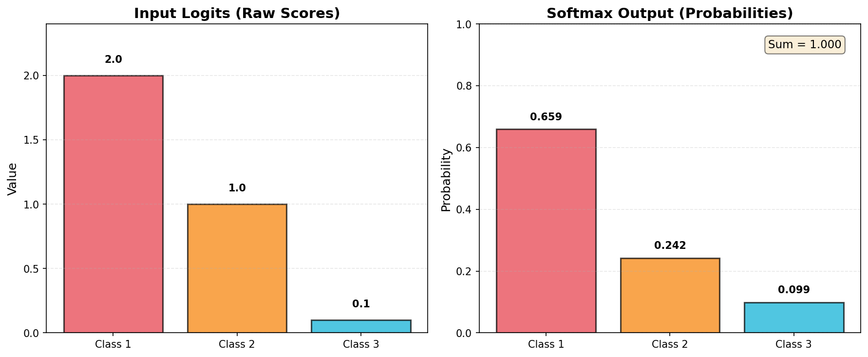
To visualize how softmax transforms raw scores into probabilities, consider this example with three classes:
The plot shows how softmax takes three input values (logits) and converts them into probabilities that sum to 1. Notice how higher input values result in higher probabilities, while maintaining the constraint that all outputs sum to exactly 1.
Key properties of softmax:
All output values are between 0 and 1.
The sum of all outputs equals 1, making it a valid probability distribution.
The function amplifies the highest input values and suppresses the lower ones.
When implementing softmax, we need to be careful about numerical stability. The exponential function can lead to extremely large numbers, potentially causing overflow. A common technique is to subtract the maximum value from all inputs before applying the exponential function, which doesn't change the final result but prevents numerical issues.
Let's implement a numerically stable softmax function:
#include <vector>#include <cmath>#include <algorithm>std::vector<std::vector<double>> softmax(const std::vector<std::vector<double>>& x) { std::vector<std::vector<double>> result(x.size()); for (size_t i = 0; i < x.size(); ++i) { result[i].resize(x[i].size()); // Find maximum value in this sample double max_val = *std::max_element(x[i].begin(), x[i].end()); // Compute exponentials with numerical stability std::vector<double> exp_vals(x[i].size()); double sum_exp = 0.0; for (size_t j = 0; j < x[i].size(); ++j) { exp_vals[j] = std::exp(x[i][j] - max_val); sum_exp += exp_vals[j]; } // Normalize to get probabilities for (size_t j = 0; j < x[i].size(); ++j) { result[i][j] = exp_vals[j] / sum_exp; } } return result;}
In this implementation:
We find the maximum value across each sample's features using std::max_element.
We subtract this maximum from each value to prevent numerical overflow.
We apply the exponential function to all adjusted values using std::exp.
We divide by the sum of these exponentials to normalize the values, ensuring they sum to 1.
This implementation handles batch processing elegantly, working with inputs of shape (n_samples, n_features) and producing outputs of the same shape, where each row sums to 1.
The linear activation function (also called the identity function) simply returns the input value unchanged. This might seem trivial, but it's extremely useful for regression problems where we want to predict unbounded continuous values.
The linear activation is defined mathematically as:
The simplicity of this function belies its importance. By using linear activation in the output layer:
Our network can produce any real number as output, not limited to a specific range.
The scale of the output directly relates to the scale of our input features and weights.
We can directly interpret the output as our predicted value.
Linear activation is ideal for regression tasks like predicting house prices, temperature, stock prices, or any other continuous value that isn't naturally bounded within a specific range.
C++
#include <string>#include <stdexcept>#include <functional>class DenseLayer {private: std::vector<std::vector<double>> weights; std::vector<double> biases; int n_inputs; int n_neurons; std::vector<std::vector<double>> output; std::string activation_fn_name; std::function<std::vector<std::vector<double>>(const std::vector<std::vector<double>>&)> activation_fn;public: DenseLayer(int n_inputs, int n_neurons, const std::string& activation_fn_name = "sigmoid") : n_inputs(n_inputs), n_neurons(n_neurons), activation_fn_name(activation_fn_name) { // Initialize weights with small random values weights.resize(n_inputs, std::vector<double>(n_neurons)); for (int i = 0; i < n_inputs; ++i) { for (int j = 0; j < n_neurons; ++j) { weights[i][j] = (static_cast<double>(rand()) / RAND_MAX) * 0.1; } } // Initialize biases to zero biases.resize(n_neurons, 0.0); // Set activation function if (activation_fn_name == "sigmoid") { activation_fn = sigmoid; } else if (activation_fn_name == "relu") { activation_fn = relu; } else if (activation_fn_name == "softmax") { activation_fn = softmax; } else if (activation_fn_name == "linear") { activation_fn = linear; } else { throw std::invalid_argument("Unsupported activation: " + activation_fn_name); } } // Forward method remains unchanged as it uses the assigned activation_fn std::vector<std::vector<double>> forward(const std::vector<std::vector<double>>& inputs) { // Implementation remains the same as before // ... (matrix multiplication and bias addition) // Then apply activation function output = activation_fn(z); return output; }};
C++
#include <iostream>#include <vector>int main() { // Create sample data for classification std::vector<std::vector<double>> X_clf = { {1.0, 0.5, -1.0, 2.0}, {-0.5, 0.0, 1.5, -2.5} }; std::cout << "Input X for classification (shape " << X_clf.size() << "x" << X_clf[0].size() << "):" << std::endl; for (const auto& row : X_clf) { for (double val : row) { std::cout << val << " "; } std::cout << std::endl; } // Create an MLP with softmax output MLP mlp_softmax; mlp_softmax.add_layer(DenseLayer(4, 8, "relu")); mlp_softmax.add_layer(DenseLayer(8, 5, "relu")); mlp_softmax.add_layer(DenseLayer(5, 3, "softmax")); // 3 classes return 0;}
C++
// Forward propagate through the networkstd::vector<std::vector<double>> out_softmax = mlp_softmax.forward(X_clf);std::cout << "Output (Softmax) (shape " << out_softmax.size() << "x" << out_softmax[0].size() << "):" << std::endl;for (const auto& row : out_softmax) { for (double val : row) { std::cout << val << " "; } std::cout << std::endl;}// Calculate and display sum of probabilities per samplestd::cout << "Sum of probs per sample: ";for (const auto& row : out_softmax) { double sum = 0.0; for (double val : row) { sum += val; } std::cout << sum << " ";}std::cout << std::endl;
Output (Softmax) (shape 2x3):0.33334939 0.33380076 0.33284985 0.33333349 0.33340775 0.33325876 Sum of probs per sample: 1 1
C++
// Create sample data for regressionstd::vector<std::vector<double>> X_reg = { {0.1, 0.2, 0.3, 0.4}};std::cout << "Input X for regression (shape " << X_reg.size() << "x" << X_reg[0].size() << "):" << std::endl;for (const auto& row : X_reg) { for (double val : row) { std::cout << val << " "; } std::cout << std::endl;}// Create an MLP with linear outputMLP mlp_linear;mlp_linear.add_layer(DenseLayer(4, 10, "relu"));mlp_linear.add_layer(DenseLayer(10, 1, "linear")); // Regression output
C++
// Forward propagate through the networkstd::vector<std::vector<double>> out_linear = mlp_linear.forward(X_reg);std::cout << "Output (Linear) (shape " << out_linear.size() << "x" << out_linear[0].size() << "):" << std::endl;for (const auto& row : out_linear) { for (double val : row) { std::cout << val << " "; } std::cout << std::endl;}
Output (Linear) (shape 1x1):0.01877798
C++
#include <vector>#include <cmath>#include <algorithm>std::vector<std::vector<double>> softmax(const std::vector<std::vector<double>>& x) { std::vector<std::vector<double>> result(x.size()); for (size_t i = 0; i < x.size(); ++i) { result[i].resize(x[i].size()); // Find maximum value in this sample double max_val = *std::max_element(x[i].begin(), x[i].end()); // Compute exponentials with numerical stability std::vector<double> exp_vals(x[i].size()); double sum_exp = 0.0; for (size_t j = 0; j < x[i].size(); ++j) { exp_vals[j] = std::exp(x[i][j] - max_val); sum_exp += exp_vals[j]; } // Normalize to get probabilities for (size_t j = 0; j < x[i].size(); ++j) { result[i][j] = exp_vals[j] / sum_exp; } } return result;}