Full Table Sales Analysis
Introduction
Welcome back to Sorting, Unique Values, and Table Analysis with NumPy. We’re at the fourth and final lesson of the course. So far, we’ve sorted values, ranked complete records, and counted distinct values. Now we’ll use these familiar NumPy tools together to analyze weekly sales for three stores.
By the end of this lesson, you’ll be able to:
- Clean a working copy of a table while keeping the raw data unchanged
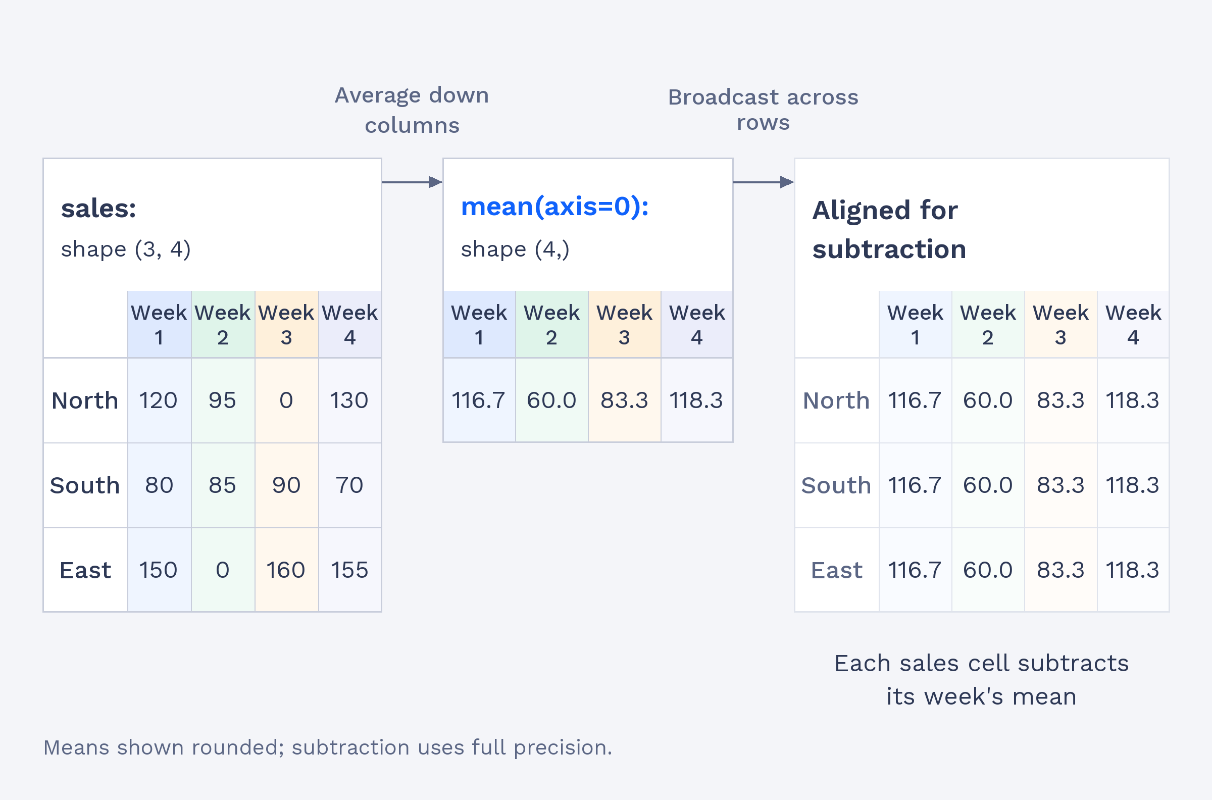
- Answer per-store and per-week questions with axis-based calculations and broadcasting
- Rank stores and filter whole rows with a combined mask
Meet the Dataset and Protect the Raw Table
We’ll start with a table whose rows represent stores and whose four columns represent weeks. The value -1 marks a missing week. Rather than changing the original data, we make a copy and replace negative values in that copy with zero. This protects raw while giving us a sales table we can calculate with. As you may recall from earlier units, a Boolean mask lets us select just the values that meet a condition.
The names in stores match the table rows in order: North, South, then East. The expression sales < 0 creates a True or False value for each cell, and the assignment changes only the cells marked True. Because sales is a copy, both -1 values remain in raw.
Replacing a missing value with zero is a simplifying assumption we make for this exercise. An unknown sales amount is not necessarily zero sales, so every total, average, and ranking below should be read as if the missing weeks had no sales. That tends to lower the totals and weekly averages of stores with missing weeks. In a real analysis, we would document a missing-data policy instead, such as leaving missing observations out of averages, reporting how many weeks were actually observed, or using a justified estimate.
Per-Store Answers with axis=1
Next, we want one total for each store. Since each store occupies a row, sum(axis=1) adds across that row. We use argmax() to find the position of the largest total, then use that position to select the store name. We can also count, for each store, how many weeks reached at least 100: the comparison creates a True or False value for each cell, and summing along axis=1 counts the True values in each row.
The output gives the best store first, followed by the count of qualifying weeks for each store in the original row order:
East has the highest total, 465. North reached 100 in two weeks, South in none, and East in three. In both calculations, axis=1 leaves us with one answer per row.